Solar Radiation Energy Analysis

Introduction

This assignment deals with an analysis of solar radiation intensity. Since solar power is more in demand than ever due to the increasing demand for renewable energy, suitable locations  have to be found. In order to find those locations, the terrain angle, exposition, shadows cast by sourrounding objects or terrain and the solar azimuth and angle need to be taken into account.
The study area is 2 square kilometers big and situated in the Salzburg area, south of the Mitterhorn mountain massif. It encopasses the village of Krallerwinkel, North-East of Maria-Alm.

DSM and Hillshade Analysis

Firstly, a 1m DSM of the area is used to create Hillshade visualizations. Since the solar radiation energy varies throughout the year, depending on the position of the sun, four different hillshade visualizations are created at the times of the equinoxes and solistices (21 January, 21 March, 21 June, 23 September, 21 December). These dates are chosen beause the solistices represent the maximum (summer) and minumum (winter) values of solar radiation, while the equinoxes show the sun’s position right in the middle of the solistice positions. Using these four dates, a good overview over the variation in solar energy throughout the year can be achieved.

The “calculate shadow” option was used, since it is of importance to see if certain areas might be blocked by sourrounding objects. The hillshade returns a raster with values ranging from 0 (complete shadow) to 255 (highest solar exposure of that day). The azimuth and angle were chosen to represent the local azimuth on the correspending day.

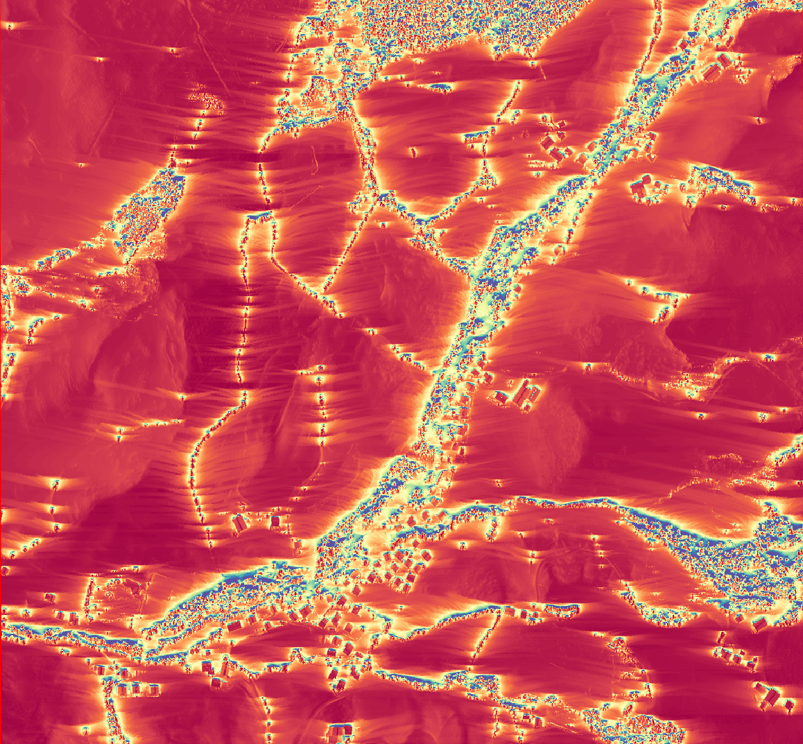
Daily Sunshine Hours and Solar Radiation Intensity

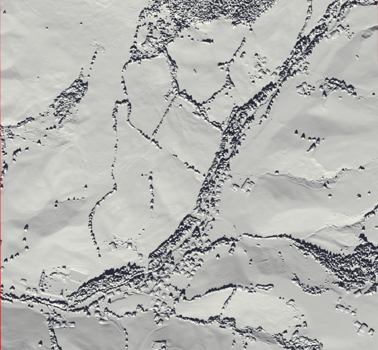
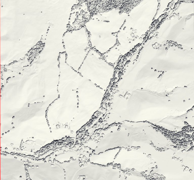
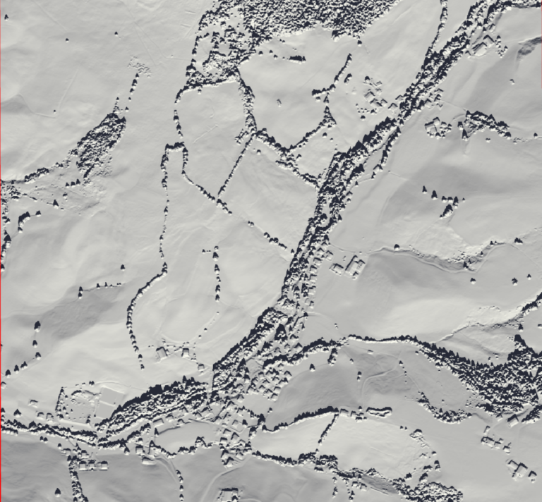
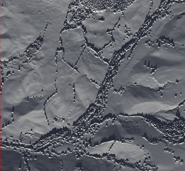
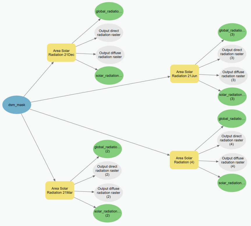
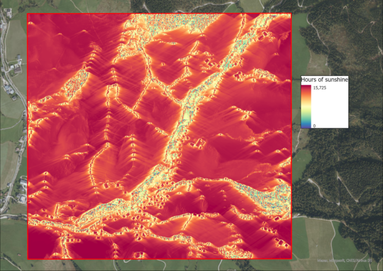
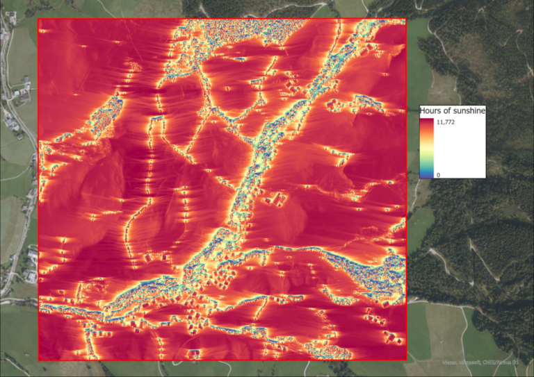
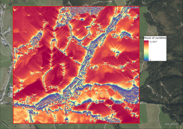
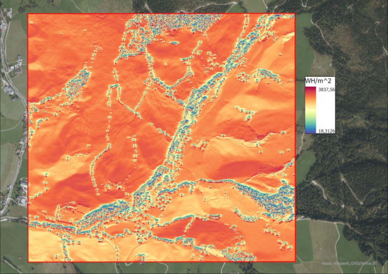
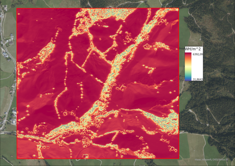
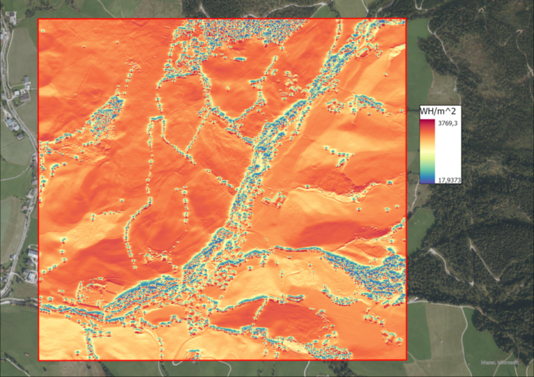
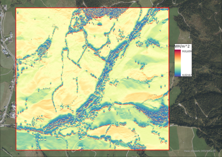
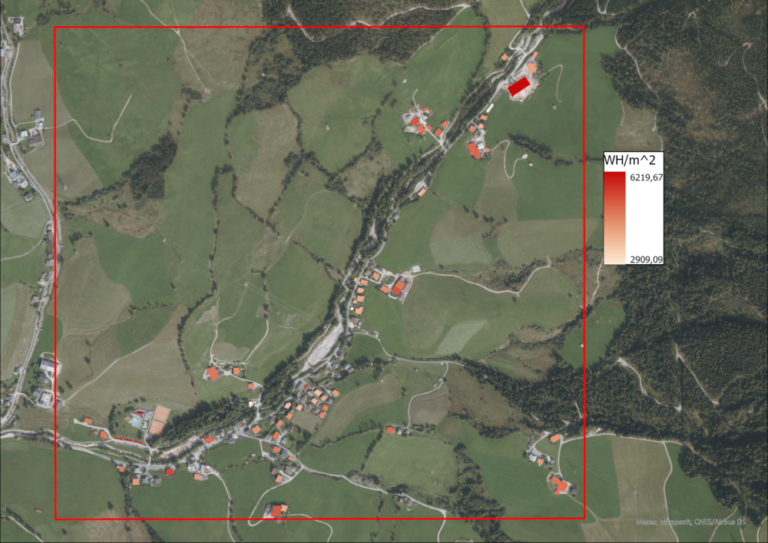
After the hillshade, the solar intensity and sunshine hours of the study region are calculated, using the “Area Solar Radiation” funciton in ArcGIS Pro. The input is the DSM, as well as the day in question. The outputs are two raster files, one containing the solar radiation intensity in Watt-hours per square meters (WH/m^2) per pixel and the other containing the hours of sunshine this pixels receives. Of course, this function is executed for each of the equinoxes and solistices.

Since the total processing time for this rather large study area and the fine 1m DSM was about 11 hours, the task was automated via the ModelBuilder in order to be able to start all 4 calculations for each date at once.

Graph 1: ModelBuilder Diagram for the “Area Solar Radiation” function.

Masking of Roofs

Since all required data to identify solar power locations have now been calculated, a layer containing most of the biggest roofs of the village and the surrounding is created. 

Image 14: Polygon layer representing roofs.

Now, the solar intensity raster is masked by the roofs in order to keep only those pixels which fall on roofs and are therefore possible solar power plant sites.

In order to identify roofs with a high potential energ yield, the zonal statistics tool is used on the WH/m^2 rasters, zoned by the roofs in pursuance of the average power yield per roof. The average roof solar yield value is assigned to each of the roof’s polygons and visualized for each point in time.

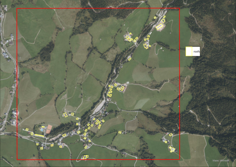
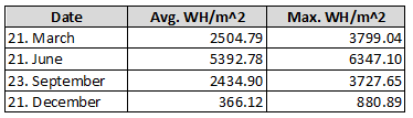
From the solar intensity raster masked by the roofs, the average and maximum power yields can also be calculated for all of the roofs combined.

Table 1: Average and maximum WH/m^2 across all roof pixels.

Identifying best suited roofs

After now knowing the average yield per roof, the top 10 roofs with the biggest yield can be identified. As a basis, the yield of the 21st of June was chosen since the highest yields occur around the summer solistice, but the result does not differ from the other dates since the yield falls and rises equally, the only difference being the angle of the roof. This does not have a big enough impact to the 10 top roofs and additionally, since the highest yields occur in summer, a higher efficiency in winter does not sufficiently increase the total year-round production.

Image 18: Top 10 roofs in red, other roofs in yellow.
Sidenote

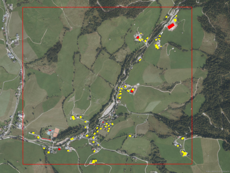
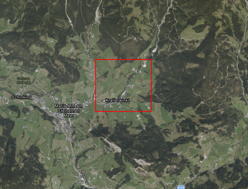
When creating the polygons, I also included some solar power plants that were already present in the area. Interestingly, these four structures are included in the top 10 roofs/structures, verifying my process and the engineers decision to build the solar power plants at these locations.

Image 20: Solar power plant already present in the AOI appear in the best performing structures.

Identifying areas of high and low radiation intensity

Additionally to the already perfomed analysis, two extra questions are posed:

  • Which field would be best suited for a sunflower field?
  • Where does the snow melt first and last?

In order to answer the first question, the area with the highest sunshine time in summer is identified. Not knowing much about the biology of the Helianthus annuus, I assume that the plant cares more about the sunshine duration in order to trigger it’s growth cycle than the actual intensity of the radiation, therefore the area with the 10 highest percent of sunshine duration in summer is identified. Those are the areas with at least 14.15 hours of sunlight.

Image 20: Highlighted in a transparent red are all those areas in the AOI, that have at least 10% of the maximum sunshine duration of the complete AOI on the summer solistice. These areas would be best for planting a sunflower field.

Next, the task is to find out where snow would melt first and last. For that, the top and bottom 10% of maximum solar radiation intensity areas of the AOI are identified, based on the solar radiation intensity of the winter solistice.

Image 21: Lowest 10% radiation areas (blue) and top 10% radiation areas (red). Quite logically, since this is a DSM, high object such as the trees have surfaces that are very inclined towards the sun, therefore receiving much more radiation than their shadows. This image is a representation of that. In order to see the snowmelt on the flat areas, the same analysis would have to be perdormed on a DEM.

Leave a Reply

Your email address will not be published. Required fields are marked *

Further Reading
Recent Updates