Introduction and Comments
This notebook is specifically structured to run/train/evaluate multiple models on the cluster. By setting the variables in the "setting" cell, it can be chosen whichmodels should be run and with wich general parameters. The logging of model information is handeld via "weights and bias". This structure has been chosen since quite a few GPU-intensive models are trained, the execution was therefore run on the university cluster instead of straiht from the notebook.
A detailed list of the models that have been run, their parameters and performance is summarized in the Report section.
Content
- Data Loading and environment setup
- Exploration
1.1 Visualization 1.2 Dataset Skewedness - Dataloader
- untrained Architechtures (trained from scrach)
3.1 Training of Models
3.2 Model Metrics3.1.1 LeNet5 3.1.2 ResNet16 3.1.2.1 ResNet16 "shallow end classifier" 3.1.2.2 ResNet16 "deep end classifier" 3.1.3 VGG18 3.1.4 Alexnet - Pretrained Archtiechtures - Transfer Leraning
4.1 VGG
4.2 ResNet - Training of best model: ResNet16 trained from scratch
- Report
6.1 Data - Quality and skewedness
6.2 untraines Models: Parameters and Performance
6.3 pretrained Models: Parameters and Performance
6.4 Final Model
6.5 Conclusion
# imports
import wandb
import os
import pandas as pd
import numpy as np
import rasterio
from prettytable import PrettyTable

from sklearn.model_selection import train_test_split
import torch
from torch.utils.data import Dataset
from torchvision.io import read_image
from torch.utils.data import DataLoader
from torchvision import datasets, transforms
from torchvision.transforms import ToTensor
import matplotlib.pyplot as plt
import random


import numpy as np
import pandas as pd
import matplotlib.pyplot as plt
from sklearn.model_selection import train_test_split

import IPython

import torch
import torch.nn as nn
import torch.nn.functional as F
import torch.optim as optim
import torchvision
from torchvision.transforms import transforms
import torchvision.datasets as datasets
from torch.utils.data import DataLoader, random_split
from torchvision.transforms import ToTensor

from torch.optim import lr_scheduler
import time
import copy
"""
SETTINGS
"""

# print and plot info
# if run inside a notebook, should be set to true
notebook = True


# choose to balance dataset
balance_dataset = True

# choose optimizer
#optim = "adam"
optim = "sdg"

# define which of the models should be run
train_rf = False # train RF
train_lenet = False # train LeNet
train_resnet = False # train resnet
train_resnet_variation2 = False # train resnet
train_vgg = False # train vgg
train_alexnet = False # train alexnet
train_vgg_pretrained = False # retrain pretrained VGG
train_resnet_pretrained = False # retran pretrained resnet
train_and_save = True # train and save final model


# set data path
local_path = "/home/simon/CDE_UBS/deep_learning/EOT/assignment"
server_path = "/share/etud/e2008983/testing/assignment"
# set datapeth depending on if ru on server or lically
if os.path.exists(local_path):
    project_path = local_path
if os.path.exists(server_path):
    project_path = server_path
Reading the data
The information on the training data is stored in the csv file traindata.csv.
train_df = pd.read_csv(os.path.join(project_path, "traindata.csv"))
if notebook:
    print(train_df)
The img_id column indicates the relative path to the image and the has_oilpalm columns give the corresponding class index.
Let us now dowload the data and train a simple Random Forest algorithm on the flatten representation of the training images. As the data are big (~12GB if we donwload them in a float64 numpy array), we will use here only a subset of the data.
#-- Training a RF model
if train_rf:

    N = 500
    #-- Getting the training dataset (X,y)
    X = np.zeros((N,256*256*3), dtype=np.uint16)
    y = np.zeros((N,), dtype=np.uint8)
    train_rf_model = train_df.sample(n=N)
    for n in range(N):
        X[n,:] = rasterio.open(os.path.join(project_path,train_rf_model.iloc[n]['img_id'])).read().flatten()
        y[n] = train_rf_model.iloc[n]['has_oilpalm']


    from sklearn.ensemble import RandomForestClassifier
    rf = RandomForestClassifier(n_estimators=100, max_features=100, max_depth=25, oob_score=True, n_jobs=-1)
    rf.fit(X,y)
    print('OOB error for unbalanced data:', rf.oob_score_)
if notebook:
from matplotlib import pyplot as plt
fig, axs = plt.subplots(10,5, figsize=(15, 30), facecolor='w', edgecolor='k')
#fig.subplots_adjust(hspace = .5, wspace=.001)
axs = axs.ravel()
count=0
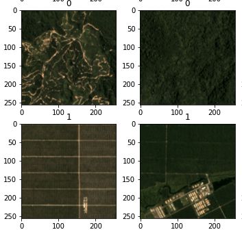
for path,typ in zip(train_df["img_id"][:50],train_df["has_oilpalm"][:50]):
src = rasterio.open(path)
b1 = src.read(1)
b2 = src.read(2)
b3 = src.read(3)
im = np.dstack((b1,b2,b3))
axs[count].imshow(im)
axs[count].set_title(str(typ))
count=count+1

1.2 Skewedness of Data
if notebook:
    train_df["has_oilpalm"].value_counts().plot(kind='bar')
    plt.title("Classes Count")
    plt.show()

if balance_dataset:
    print("Balancing Dataset - Random undersampling")

    # Class count
    count_class_0, count_class_1 = train_df.has_oilpalm.value_counts()

    # Divide by class
    df_class_0 = train_df[train_df['has_oilpalm'] == 0]
    df_class_1 = train_df[train_df['has_oilpalm'] == 1]

    df_class_0_under = df_class_0.sample(count_class_1)
    train_df = pd.concat([df_class_0_under, df_class_1], axis=0)


    print(train_df.has_oilpalm.value_counts())
    train_df["has_oilpalm"].value_counts().plot(kind='bar')
    plt.title("Classes Count")
    plt.show()

The dataset is quite skewed. Assigning all samples the prediction "0" would already lead to results in the 0.85 percent range, which will hinder identification of suitable models.
An undersampling method was implemented to balance the dataset if desired. While some information is lost due to the removal of samples, the features that we want to detect are in the minority class. Therefore, the variance in the features that decide on the class in not reduced, only the other samples are removed. Implementing oversampling would have significantly inreased the training time and would have not added any new information or benefit over undersampling. Still, calculations will be done on both datasets.
2. Build DataLoaders
# perform train test split, which is stratified
train_split,test_split = train_test_split(train_df,test_size=0.25, random_state=42,stratify=train_df["has_oilpalm"])
if notebook:
    train_split["has_oilpalm"].value_counts().plot(kind='bar')
    plt.title("Train Dataset")
    plt.show()
    test_split["has_oilpalm"].value_counts().plot(kind='bar')
    plt.title("Test Dataset")
    plt.show()
# Define Transformer

# transform = transforms.ToTensor()

transform = transforms.Compose([
    #transforms.ToTensor(),
    #transforms.Resize((256,256)),
    #transforms.ConvertImageDtype(torch.float),
    transforms.Normalize((0.4914, 0.4822, 0.4465), (0.2023, 0.1994, 0.2010))
])
class Dataset(Dataset):
    def __init__(self,dataset,transform):
        # extract x and y as lists from DF
        self.x = dataset["img_id"].tolist()
        self.y = dataset["has_oilpalm"].tolist()
        self.transform = transform

    def __len__(self):
        # returns length
        return len(self.x)

    def __getitem__(self,idx):
        # read image with tensor io
        im = read_image(self.x[idx])
        im = im.type(torch.DoubleTensor) # change data type to double
        # transform if var set
        if self.transform:
            im = self.transform(im)
        # read y from list
        y = self.y[idx]
        # return as tuple
        return(im,y)

dataset_train = Dataset(train_split,transform=transform)
dataset_test  = Dataset(test_split,transform=transform)
dataset_full  = Dataset(train_df,transform=transform)

print("Length DataSet Object Train : ",dataset_train.__len__())
print("Length DataSet Object Test  : ",dataset_test.__len__())
print("Length DataSet Object Full  : ",dataset_full.__len__())
# create loaders

#loader_train = DataLoader(dataset_train,batch_size=16, shuffle=True, num_workers=5)
#loader_test  = DataLoader(dataset_test,batch_size=16, shuffle=True, num_workers=5)
#loader_full  = DataLoader(dataset_test,batch_size=16, shuffle=True, num_workers=5)

# loaders are initialized in train_model function based on batch size specified
3. Try various architechtures of untrained models
Several architechtures are loaded and trained from scratch. The idea is to find out if a model is well adapted to the task, not to perform any kind of prediction. Later on, when suitable models have been found and their hyperparameters tested, the predictions will be performed. Please note that the models are not trained from this notebook here, but on the volta1 server.
def count_parameters(LeNet5):
    table = PrettyTable(["Modules", "Parameters"])
    total_params = 0
    for name, parameter in model.named_parameters():
        if not parameter.requires_grad: continue
        param = parameter.numel()
        table.add_row([name, param])
        total_params+=param
    print(table)
    print(f"Total Trainable Params: {total_params}")
# implementation of model trainer function
def train_model(model,batch_size,lr,epochs,wandb_name):

    # configure logging

    # "eot_deep-learning-LeNet"
    # "eot_deep-learning-ResNet"
    # "eot_deep-learning-vgg"
    # "eot_deep-learning-inc"
    wandb.init(project=wandb_name, entity="simon-donike")

    wandb.config = {
      "learning_rate": lr,
      "epochs": epochs,
      "batch_size": batch_size
    }

    # define loaders
    loader_train = DataLoader(dataset_train,batch_size=batch_size, shuffle=True, num_workers=5)
    loader_test  = DataLoader(dataset_test,batch_size=batch_size, shuffle=True, num_workers=5)
    loader_full  = DataLoader(dataset_test,batch_size=batch_size, shuffle=True, num_workers=5)


    train_loss = []  # where we keep track of the training loss
    train_accuracy = []  # where we keep track of the training accuracy of the model
    val_loss = []  # where we keep track of the validation loss
    val_accuracy = []  # where we keep track of the validation accuracy of the model
    epochs = epochs  # number of epochs

    # initialize model

    model = model.double()

    model.to(device)
    if optim = "sdg":
        optimizer = optim.SGD(model.parameters(), lr=lr)
    if optim = "adam"
        optimizer = optim.Adam(model.parameters(), lr=lr)

    for e in range(epochs):
        model.train()
        train_correct = 0
        for (x_train_batch, y_train_batch) in loader_train:
            x_train_batch = x_train_batch.to(device)

            # y_train_batch = y_train_batch.to(torch.int32) # convert to torch int

            y_train_batch = y_train_batch.to(device)

            y_hat = model(x_train_batch)  # forward pass

            loss = loss_func(y_hat, y_train_batch)  # compute the loss

            loss.backward()  # obtain the gradients with respect to the loss
            optimizer.step()  # perform one step of gradient descent
            optimizer.zero_grad()  # reset the gradients to 0
            y_hat_class = torch.argmax(y_hat.detach(), axis=1)  # we assign an appropriate label based on the network's prediction
            train_correct += torch.sum(y_hat_class == y_train_batch)
            train_loss.append(loss.item() / len(x_train_batch))
            wandb.log({'loss': loss.item() / len(x_train_batch)})

        train_accuracy.append(train_correct / len(loader_train.dataset))
        wandb.log({'train_acc': train_correct / len(loader_train.dataset)})


        model.eval()  # notify all the layers that you are in eval mode (useful for batch norm, dropout, etc)
        tmp_val_loss = 0
        val_correct = 0
        with torch.no_grad():  # ....impacts the autograd engine and deactivate it.

            # reduce memory usage and speed up computations.

            for (x_val_batch, y_val_batch) in loader_train:
                x_val_batch = x_train_batch.to(device)
                y_val_batch = y_train_batch.to(device)
                y_val_hat = model(x_val_batch)  # forward pass
                tmp_val_loss += loss_func(y_val_hat, y_val_batch).item()  # compute the loss
                y_val_hat_class = torch.argmax(y_val_hat.detach(), axis=1)  # we assign an appropriate label based on the network's prediction
                val_correct += torch.sum(y_val_hat_class == y_val_batch)
        val_loss.append(tmp_val_loss / len(loader_train.dataset))  # compute the average loss....
        val_accuracy.append(val_correct / len(loader_train.dataset))
        wandb.log({'val_acc': val_correct / len(loader_train.dataset)})
        print ('Epoch', e+1, ' finished.')

    wandb.finish()
# NN architecture
class LeNet5(nn.Module):
    def __init__(self, n_channels, n_classes):
        super(LeNet5, self).__init__()
        #-- convolutional layers
        self.conv1 = nn.Conv2d(n_channels, 6, 5)
        self.conv2 = nn.Conv2d(6, 16, 5)
        self.conv3 = nn.Conv2d(16, 120, 5)

        #-- fully connected layers
        self.fc1 = nn.Linear(120*28*28, 84)
        self.fc2 = nn.Linear(84, n_classes)

    def forward(self, x):
        x = F.max_pool2d(F.relu(self.conv1(x)), 2)
        x = F.max_pool2d(F.relu(self.conv2(x)), 2)
        x = F.max_pool2d(F.relu(self.conv3(x)), 2)
        # flatten all dimensions except the batch dimension
        x = torch.flatten(x, start_dim=1)
        x = F.relu(self.fc1(x))
        logits = self.fc2(x)
        return logits


# Loss function
def loss_func(y_hat, y):
    return nn.CrossEntropyLoss()(y_hat, y)

device = torch.device("cuda:0" if torch.cuda.is_available() else "cpu")
print("Running on:",device)
if train_lenet:
    model = LeNet5(3,2)
    count_parameters(model)
    train_model(model,16,0.01,25,"eot_deep-learning-LeNet_v2")
3.1.2 try untrained ResNet - balanced and unbalanced Datasets
3.1.2.1 ResNet shallow end
if train_resnet:
    #model = torch.hub.load('pytorch/vision:v0.10.0', 'resnet18', pretrained=False)
    model = torchvision.models.resnet18(pretrained=False)

    print("original model")
    count_parameters(model)

    # reconfigure last layers to fit data
    model.fc = torch.nn.Linear(in_features=512, out_features=2, bias=True)


    print("\nreconfigured model")
    count_parameters(model)
if train_resnet:
    # train_model(model,batch_size,lr,epochs,wandb_name):
    #train_model(model,32,0.001,20,"eot_deep-learning-ResNet")
    #print("ResNet 1 finished")
    train_model(model,32,0.0001,50,"eot_deep-learning-ResNet_v2")
    #print("ResNet 2 finished")
    #train_model(model,16,0.00001,20,"eot_deep-learning-ResNet")
    #print("ResNet 3 finished")
Best Result: Resnet 0.0001_32
3.1.3.2 ResNet Deep End
if train_resnet_variation2:
    #model = torch.hub.load('pytorch/vision:v0.10.0', 'resnet18', pretrained=False)
    model = torchvision.models.resnet18(pretrained=False)

    print("original model")
    count_parameters(model)

    # reconfigure last layers to fit data
    model.fc = torch.nn.Sequential(
    torch.nn.Linear(in_features=512, out_features=128, bias=True),
    torch.nn.Linear(in_features=128, out_features=64, bias=True),
    torch.nn.Linear(in_features=64, out_features=2, bias=True))

    print("\nreconfigured model")
    count_parameters(model)
if train_resnet_variation2:
    print("ResNet Deep End: training")
    train_model(model,32,0.0001,50,"eot_deep-learning-ResNet_v2")
3.1.3 try untrained VGG - unbalanced dataset
if train_vgg:
    #model = torch.hub.load('pytorch/vision:v0.10.0', 'resnet18', pretrained=False)
    model = torchvision.models.vgg16(pretrained=False)
    print("predefined model")
    count_parameters(model)


    model.classifier = torch.nn.Sequential(
    torch.nn.Linear(in_features=25088, out_features=4096, bias=True),
    torch.nn.ReLU(inplace=True),
    torch.nn.Dropout(p=0.5, inplace=False),
    torch.nn.Linear(in_features=4096, out_features=2048, bias=True),
    torch.nn.ReLU(inplace=True),
    torch.nn.Dropout(p=0.5, inplace=False),
    torch.nn.Linear(in_features=2048, out_features=2, bias=True) )

    print("\nadapted model")
    count_parameters(model)
if train_vgg:
    train_model(model,32,0.001,10,"eot_deep-learning-VGG_v2")
    print("VGG-1 completed")
3.1.4 try untrained alexnet - unbalanced dataset
if train_alexnet:
    model = torchvision.models.alexnet(pretrained=False)
    print("predefined model")
    count_parameters(model)

    model.classifier = torch.nn.Sequential(
    torch.nn.Dropout(p=0.5, inplace=False),
    torch.nn.ReLU(inplace=True),
    torch.nn.Dropout(p=0.5, inplace=False),
    torch.nn.Linear(in_features=4096, out_features=4096, bias=True),
    torch.nn.ReLU(inplace=True),
    torch.nn.Dropout(p=0.5, inplace=False),
    torch.nn.Linear(in_features=2048, out_features=2, bias=True) )

    print("\n adapted model")
    count_parameters(model)
if train_alexnet:
    # vgg 1
    train_model(model,16,0.001,50,"eot_deep-learning-alex_v2")
    print("inception_v3 1 completed")

    # vgg 2
    train_model(model,16,0.0001,50,"eot_deep-learning-alex_v2")
    print("inception_v3 2 completed")
3.2 Info on Models
3.2.1 - LeNet
url = "https://wandb.ai/simon-donike/eot_deep-learning_LeNet/reports/LeNet-Report--VmlldzoxNDQxNDg5?accessToken=ue91g0soke14ynh67aldbwsfh0t65o10b0khqb4szpojodn92iftrh722rb7p4ow"
iframe = '<iframe src=' + url + ' width=800 height=600></iframe>'
IPython.display.HTML(iframe)
3.2.2 - ResNet
url = "https://wandb.ai/simon-donike/eot_deep-learning-ResNet/reports/Untrained-ResNet-Report--VmlldzoxNDQxNDQ1?accessToken=b300jbobd5mr4f1f9ynyx72rip7kyhs5kzr15jlng124p0hgzojjpn7vagpefj0l"
iframe = '<iframe src=' + url + ' width=800 height=600></iframe>'
IPython.display.HTML(iframe)
url = "https://wandb.ai/simon-donike/eot_deep-learning-ResNet_v2/reports/ResNet-optimized--VmlldzoxNDQ0ODUz?accessToken=07hro4sq0j8nc149utj51xteu8qw207kjm0vxg6eyu6185r5gnls53kkeuz3yab6"
iframe = '<iframe src=' + url + ' width=800 height=600></iframe>'
IPython.display.HTML(iframe)
3.2.3 - VGG
url = "https://wandb.ai/simon-donike/eot_deep-learning-VGG/reports/Untrained-VGG16-Report--VmlldzoxNDQxNDkw?accessToken=ro5f4qohu5ajgxr1gex32lwcxsf4400hc78647870hahyct5jsvcaz4sighc592p"
iframe = '<iframe src=' + url + ' width=800 height=600></iframe>'
IPython.display.HTML(iframe)
3.2.4 - AlexNet
url = "https://wandb.ai/simon-donike/eot_deep-learning-alex/reports/Untrained-AlexNet-Report--VmlldzoxNDQxNDk4?accessToken=n5o5456x62i2dm7883ac8h4mtp498n2756p1q2zrynkmesqxe0kn63q0w5i06gvm"
iframe = '<iframe src=' + url + ' width=800 height=600></iframe>'
IPython.display.HTML(iframe)
4. Transfer Learning: Run on pretrained model
Since VGG is the most complex model and ResNet yields the best results so far, it might be useful to try these pretrained models. Even though they have been trained from scratch previously, model performance might benefit from having several layers pretrained on other data, which can then detect certain features in the images. This way, the pretrained models might be useful for feature extraction.
Following tutorial: https://pytorch.org/tutorials/beginner/transfer_learning_tutorial.html
4.1 Pretrained VGG
# implementation of model trainer function
def train_pretrained_model(model,batch_size,lr,epochs,wandb_name):

    # configure logging

    # "eot_deep-learning-LeNet"
    # "eot_deep-learning-ResNet"
    # "eot_deep-learning-vgg"
    # "eot_deep-learning-inc"
    wandb.init(project=wandb_name, entity="simon-donike")

    wandb.config = {
      "learning_rate": lr,
      "epochs": epochs,
      "batch_size": batch_size
    }

    # define loaders
    loader_train = DataLoader(dataset_train,batch_size=batch_size, shuffle=True, num_workers=5)
    loader_test  = DataLoader(dataset_test,batch_size=batch_size, shuffle=True, num_workers=5)
    loader_full  = DataLoader(dataset_test,batch_size=batch_size, shuffle=True, num_workers=5)
    print("len loader train:",len(loader_train))
    print("len loader test :",len(loader_test))

    train_loss = []  # where we keep track of the training loss
    train_accuracy = []  # where we keep track of the training accuracy of the model
    val_loss = []  # where we keep track of the validation loss
    val_accuracy = []  # where we keep track of the validation accuracy of the model
    epochs = epochs  # number of epochs

    # initialize model

    model = model.double()

    model.to(device)
    #optimizer = optim.SGD(model.parameters(), lr=lr)
    optimizer = optim.SGD(filter(lambda p: p.requires_grad, model.parameters()),lr=lr)
    for e in range(epochs):
        model.train()
        train_correct = 0
        for (x_train_batch, y_train_batch) in loader_train:
            x_train_batch = x_train_batch.to(device)

            # y_train_batch = y_train_batch.to(torch.int32) # convert to torch int

            y_train_batch = y_train_batch.to(device)

            y_hat = model(x_train_batch)  # forward pass

            loss = loss_func(y_hat, y_train_batch)  # compute the loss

            loss.backward()  # obtain the gradients with respect to the loss
            optimizer.step()  # perform one step of gradient descent
            optimizer.zero_grad()  # reset the gradients to 0
            y_hat_class = torch.argmax(y_hat.detach(), axis=1)  # we assign an appropriate label based on the network's prediction
            train_correct += torch.sum(y_hat_class == y_train_batch)
            train_loss.append(loss.item() / len(x_train_batch))
            wandb.log({'loss': loss.item() / len(x_train_batch)})

        train_accuracy.append(train_correct / len(loader_train.dataset))
        wandb.log({'train_acc': train_correct / len(loader_train.dataset)})


        model.eval()  # notify all the layers that you are in eval mode (useful for batch norm, dropout, etc)
        tmp_val_loss = 0
        val_correct = 0
        with torch.no_grad():  # ....impacts the autograd engine and deactivate it.

            # reduce memory usage and speed up computations.

            for (x_val_batch, y_val_batch) in loader_train:
                x_val_batch = x_train_batch.to(device)
                y_val_batch = y_train_batch.to(device)
                y_val_hat = model(x_val_batch)  # forward pass
                tmp_val_loss += loss_func(y_val_hat, y_val_batch).item()  # compute the loss
                y_val_hat_class = torch.argmax(y_val_hat.detach(), axis=1)  # we assign an appropriate label based on the network's prediction
                val_correct += torch.sum(y_val_hat_class == y_val_batch)
        val_loss.append(tmp_val_loss / len(loader_train.dataset))  # compute the average loss....
        val_accuracy.append(val_correct / len(loader_train.dataset))
        wandb.log({'val_acc': val_correct / len(loader_train.dataset)})
        print ('Epoch', e+1, ' finished.')

    wandb.finish()
# LOAD AND ADAPT MODEL
if train_vgg_pretrained:
    #model = torch.hub.load('pytorch/vision:v0.10.0', 'resnet18', pretrained=False)
    model = torchvision.models.vgg16(pretrained=True)

    print("pretrained model parameters:")
    count_parameters(model)

    # adapt last layers to data
    model.classifier = torch.nn. Sequential(
    torch.nn.Linear(in_features=25088, out_features=4096, bias=True),
    torch.nn.ReLU(inplace=True),
    torch.nn.Dropout(p=0.5, inplace=False),
    torch.nn.Linear(in_features=4096, out_features=1024, bias=True),
    torch.nn.ReLU(inplace=True),
    torch.nn.Dropout(p=0.5, inplace=False),
    torch.nn.Linear(in_features=1024, out_features=2, bias=True) )
    count_parameters(model)
    print("adapted pretrained model")
    count_parameters(model)

    # FREEZE LAYERS
    count=0
    for param in model.parameters():
        count=count+1
        #print(count)
        param.requires_grad = False
        if count==26:
            break
    print("Trainable parameters after freezing:")
    count_parameters(model)

    model = model.to(device)
# RUN TRAINING
if train_vgg_pretrained:
    train_pretrained_model(model,batch_size=16,lr=0.001,epochs=50,wandb_name="eot_deep-learning-VGG_pretrained")
url = "https://wandb.ai/simon-donike/eot_deep-learning-VGG_pretrained/reports/Pretrained-VGG--VmlldzoxNDQ0ODE0?accessToken=ign43l74j3xnsel4r4jng8cj8ingr129mwdcz0mzk3gl5ckx9d3n6zqodw9tpgm6"
iframe = '<iframe src=' + url + ' width=800 height=600></iframe>'
IPython.display.HTML(iframe)
4.2 pretrained ResNet
# LOAD AND ADAPT MODEL
if train_resnet_pretrained:
    model = torchvision.models.resnet18(pretrained=True)


    # define fitting transformer as required by resnet
    transform = transforms.Compose([
    #transforms.Resize(256),
    #transforms.CenterCrop(224),
    #transforms.ToTensor(),
    transforms.Normalize(mean=[0.485, 0.456, 0.406], std=[0.229, 0.224, 0.225])])
    dataset_train = Dataset(train_split,transform=transform)
    dataset_test  = Dataset(test_split,transform=transform)


    # adapt last layers to data
    model.fc = torch.nn.Sequential(
    torch.nn.Linear(in_features=512, out_features=256, bias=True),
    torch.nn.Linear(in_features=256, out_features=64, bias=True),
    torch.nn.Linear(in_features=64, out_features=2, bias=True))
    print("adapted pretrained model")
    count_parameters(model)


    # FREEZE LAYERS
    count=0
    for param in model.parameters():
        count=count+1
        #print(count)
        param.requires_grad = False
        if count==60:
            break
    print("Trainable parameters after freezing:")
    count_parameters(model)
    model = model.to(device)
# RUN TRAINING
if train_resnet_pretrained:
    train_pretrained_model(model,batch_size=16,lr=0.0001,epochs=100,wandb_name="eot_deep-learning-ResNet_pretrained")
url = "https://wandb.ai/simon-donike/eot_deep-learning-ResNet_pretrained/reports/Pretrained-ResNet-18--VmlldzoxNDQ0Njkw?accessToken=eamk2zzguxpvkq4obon6a077p2qcl8ydhjm710hc07hv1v2o5l9dc1jzh7wjybea"
iframe = '<iframe src=' + url + ' width=800 height=600></iframe>'
IPython.display.HTML(iframe)
5. Training of best model
In the previous cells, the experiments have shown that a untrained ResNet18 with a "shallow" MLP classifier structure at the end yields the best results. Based on this knowledge, a model is trained. To optimize the performance on the unseen dataset, the model is trained on all of the available data, without a previous train/test split.
def train_epoch(model, optimizer, loss_func, dataloader, device):
    model.train()
    train_correct = 0
    train_loss = []
    for x_train_batch, y_train_batch in dataloader:
        x_train_batch = x_train_batch.to(device)
        y_train_batch = y_train_batch.to(device)

        y_hat = model(x_train_batch) # forward pass

        loss = loss_func(y_hat, y_train_batch) # compute the loss

        loss.backward() # obtain the gradients with respect to the loss
        optimizer.step() # perform one step of gradient descent
        optimizer.zero_grad() # reset the gradients to 0
        y_hat_class = torch.argmax(y_hat.detach(), axis=1) # we assign an appropriate label based on the network's prediction
        train_correct += torch.sum(y_hat_class==y_train_batch)
        train_loss.append(loss.item()/len(x_train_batch))
        wandb.log({'loss': loss.item()/len(x_train_batch)})

    train_accuracy = train_correct/len(dataloader.dataset)
    return train_loss, train_accuracy

def val_epoch(model, loss_func, dataloader, device):
    model.eval()
    tmp_val_loss = 0
    val_correct = 0
    with torch.no_grad():
        for x_val_batch, y_val_batch in dataloader:
            x_val_batch = x_val_batch.to(device)
            y_val_batch = y_val_batch.to(device)
            y_val_hat = model(x_val_batch) # forward pass
            tmp_val_loss += loss_func(y_val_hat, y_val_batch).item() # compute the loss
            y_val_hat_class = torch.argmax(y_val_hat.detach(), axis=1) # we assign an appropriate label based on the network's prediction
            val_correct += torch.sum(y_val_hat_class==y_val_batch)
    val_loss = tmp_val_loss/len(dataloader.dataset) # compute the average loss
    val_accuracy = val_correct/len(dataloader.dataset)

    return val_loss, val_accuracy
# implementation of model trainer function


def train_and_save_model(model,batch_size,lr,epochs,wandb_name):

    wandb.init(project=wandb_name, entity="simon-donike")

    wandb.config = {
      "learning_rate": lr,
      "epochs": epochs,
      "batch_size": batch_size
    }

    loader_train = DataLoader(dataset_train,batch_size=batch_size, shuffle=True, num_workers=5)
    loader_test  = DataLoader(dataset_test,batch_size=batch_size, shuffle=True, num_workers=5)

    train_loss = [] # where we keep track of the training loss
    train_accuracy = [] # where we keep track of the training accuracy of the model
    val_loss = [] # where we keep track of the validation loss
    val_accuracy = [] # where we keep track of the validation accuracy of the model
    epochs = epochs # number of epochs

    model = model.double()
    model.to(device)
    optimizer = optim.Adam(model.parameters(), lr=lr)

    min_val_loss = np.Inf
    max_val_accuracy = 0
    counter = 0
    patience = 4 #-- how long to wait after last time validation loss improved
    delta_p = 0 #-- minimum change required in the monitored quantity (e.g. validation loss) to qualify as an improvement
    for e in range(epochs):
        epoch_train_loss, epoch_train_accuracy = train_epoch(model, optimizer, loss_func, loader_train, device)
        epoch_val_loss, epoch_val_accuracy = val_epoch(model, loss_func, loader_test, device)

        #wandb.log({'loss': epoch_train_loss})
        train_loss.extend(epoch_train_loss)
        train_accuracy.append(epoch_train_accuracy)
        wandb.log({'train_acc': epoch_train_accuracy})
        val_loss.append(epoch_val_loss)
        val_accuracy.append(epoch_val_accuracy)
        wandb.log({'val_acc': epoch_val_accuracy})
        #if epoch_val_loss < min_val_loss:
        if epoch_val_accuracy > max_val_accuracy:
            #min_val_loss = epoch_val_loss
            max_val_accuracy = epoch_val_accuracy
            counter = 0
            print("saved model in epoch: ",e+1)
            torch.save({'epoch': e,
                'model_state_dict': model.state_dict(),
                'optimizer_state_dict': optimizer.state_dict(),
                'loss': epoch_train_loss
                }, "oilpalm_model.pth")
        elif epoch_val_loss-min_val_loss > delta_p:
            counter = counter + 1

        if counter == patience:
            break
        print("Epoch",e+1,"finished")
if train_and_save:
    #model = torch.hub.load('pytorch/vision:v0.10.0', 'resnet18', pretrained=False)
    model = torchvision.models.resnet18(pretrained=False)
    print("original model")
    count_parameters(model)
    # reconfigure last layers to fit data
    model.fc = torch.nn.Linear(in_features=512, out_features=2, bias=True)
    print("\nreconfigured model")
    count_parameters(model)
    train_and_save_model(model,12,0.0001,50,"eot-deep_learning_final")
url = "https://wandb.ai/simon-donike/eot-deep_learning_final/reports/Final-Model-Training--VmlldzoxNDQ2NDc5?accessToken=qls9qe9kslk9r1kgeqwgsges2pfxkwuoyd1zwjh6h49euk1xlkl3zd7w4qlk0o6d"
iframe = '<iframe src=' + url + ' width=800 height=600></iframe>'
IPython.display.HTML(iframe)
6. Report
The general philosophy behind tackling the problem in this asignment is based on pre-existing models. As seen in the LeNet example, smaller Networks are not able to perform very well, most likely because they are not deep enough to accurately represent the differences inherent in the two classes. The usage of deeper, predefined models chosen because the general distinction between simple lines and crosses (characteristic roadnetwork of plantations) is not sufficient, because many images have inhabitet areas with similar roadnetworks on them. The usage of deeper models hopefully enables the distinction between characteristics of the plant/rainforest canopy itself, instead of relying too much on roads.
The models are trained from scratch in the first step, and then the pretrained weights are loaded and only the last classifier layers redefined and trained in order to benefit from transfer learning, where the feature extraction is handled by the pretrained network and the classifier trained on these features.
6.1 Data - Quality and Skewedness
The dataset consits of only 7677 images. the dataset is very skewed, with 6722 images showing no palm oil trees and 955 images showing palm trees (see 1.2.). Other than the skewedness of the data, the quality is also quite poor. Some images labeled as "1" clearly have no palm trees, while other images labeld as "1" have only very small sections of the image covered by plantations (See 1.1).
The models were trained on the whole dataset and additionally retrained with a clean dataset, where skewedness was handled by undersampling the majority class. Oversampling the minority class would have intensified the problems in the dataset in my opinion.
6.2 Untrained Models
The following architectures were retrained from scratch. The best-performing settings per model are marked with a ✔️:
- LeNet5:
- optimizers:
- SDG ✔️
- ADAM
- learning Rates:
- 0.01
- 0.001 ✔️
- Datasets:
- balanced ✔️
- unbalanced
- BEST RESULT:
- Validation Accuracy 0.4 on unbalanced data
- COMMENT:
- while fast, the model is not suited to this problem and actualy worse than guessing.
- optimizers:
- Resnet18:
- optimizers:
- SDG ✔️
- ADAM
- learning Rates:
- 0.01
- 0.001
- 0.0001 ✔️
- 0.00001
- batch Sizes:
- 16 ✔️
- 32
- Datasets:
- balanced ✔️
- unbalanced
- Final Classifier structure:
- "Shallow End": 1 FC layer ✔️
- "Deep End": 3 FC layers
- BEST RESULT:
- Validation Accuracy 0.80 on balanced data
- COMENTS:
- sweet spot between too slow and too fast, comparatively high accuracy.
- optimizers:
- VGG16:
- optimizers:
- SDG ✔️
- learning rates:
- 0.001 ✔️
- batch size:
- 32
- datasets:
- unbalanced ✔️
- BEST RESULT:
- Validation Accuracy 0.90 on unbalanced data
- COMMENTS:
- very large, slow network. Boost in accuracy does not justify increased processing time. only tested on unbalanced data, not comparable to other models.
- optimizers:
- AlexNet:
- optimizers:
- SDG ✔️
- ADAM
- Learning Rates:
- 0.001 ✔️
- 0.0001
- Batch Size
- 16 ✔️
- Dataset:
- balanced ✔️
- unbalanced
- BEST RESULT
- Validation Accuracy 0.81 on unbalanced dataset, 0.50 on balanced data
- COMMENTS
- quick to train, but no convergence.
- optimizers:
6.3 Pretrained Models
- VGG16:
- optimizers:
- SDG ✔️
- learning rates:
- 0.001
- 0.0001
- unfrozen layers
- 3 FC classifier layers ✔️
- BEST RESULT:
- Validation Accuracy 0.5 on balanced dataset
- COMMETN:
- Transfer learning failed. Slow process.
- optimizers:
- ResNet18:
- Optimizers:
- SDG ✔️
- ADAM
- Learning rates:
- 0.001
- 0.0001 ✔️
- Batch Sizes:
- 16 ✔️
- unfrozen Layers:
- all 3 FC classifier layers ✔️
- only 2 FC classifier layers
- BEST RESULT:
- Validation Accuracy 0.5 on balanced dataset
- COMMENT:
- transfer learning failed.
- Optimizers:
6.4 Final Model
Based on the previous experiments, the following model was chosen:
- ResNet 18
- optimizer: SDG
- dataset: balanced
- learning rate: 0.0001
- batch size: 16
- patience: 4 epochs on val_accuracy
- Classifier Archtiecture: Shallow end, 1 FC layer
The final validation performance is 0.80. While there is room for improvement, overfitting is very likely to occur with continued training. The accuracy is quite low due to the smaller dataset of the balanced images and the low quality of the input data, but the model will hopefully be able to generalize better than other models.
6.5 Conclusion
In total, 34 models with different architechtures, datasets and parameters were run. The validation accuracy for all of models are quite low. No model converged to a satisfying degree, most likely due to the dataset. My aim was to try out predefined architectures and transfer learning. While I was able to learn a lot, not focussing too much on these architectures and potentially defining my own architectures would have been interesting aswell. Another thing I would have liked to try was improving the dataset, like different weights for the loss functions of the classes or data augmentation techniques for the minority class. Unfortunately I could not try out these methods.
Still, from all the models and parameters that were tried, the final result hopefully is able to generalize well, even if the accuracy is not too high.