In [1]:
from skimage import io
from skimage import color
from skimage.restoration import denoise_nl_means, estimate_sigma
import numpy as np
from numpy.fft import fft, fftfreq, ifft
from scipy import ndimage as nd
from scipy.fft import fft, ifft
from scipy import fftpack
from PIL import Image, ImageDraw
import matplotlib.pyplot as plt
import time
import cv2
from math import sqrt
from math import exp
1.1 Load an image
In [2]:
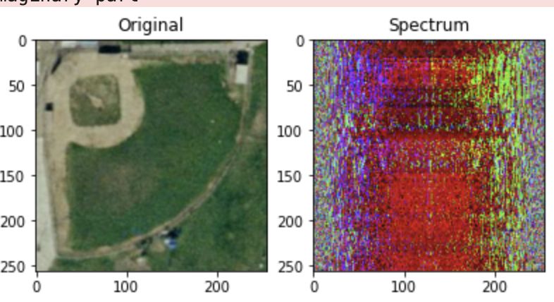
img = io.imread("images/baseballdiamond08.tif")
plt.imshow(img)
plt.show()

1.2 Verify the invertibility of the FFT
In [3]:
# https://scipy-lectures.org/intro/scipy/auto_examples/solutions/plot_fft_image_denoise.html
# fft
img_fft = fftpack.fft2(img)
# inverse of signal
img_ifft = fftpack.ifft2(img_fft).real
plt.figure(figsize=(10,10))
plt.subplot(131)
plt.imshow(img)
plt.title("Original")
plt.subplot(132)
plt.title("Spectrum")
plt.imshow(img_fft.astype(np.uint8))
plt.subplot(133)
plt.title("Reconstructed")
plt.imshow(img_ifft.astype(np.uint8))
plt.show()

The reconstruction based on the spectrum returns the original image.
In [4]:
def rgb2gray(rgb):
return np.dot(rgb[...,:3], [0.2989, 0.5870, 0.1140])
img = rgb2gray(img)
plt.imshow(img,cmap="gray")
plt.title("Gray")
plt.show()

In [5]:
plt.figure(figsize=(8, 6), constrained_layout=False)
img_fft = np.fft.fft2(img)
img_fftshift = np.fft.fftshift(img_fft)
img_ifftshit = np.fft.ifftshift(img_fftshift)
img_ifft = np.fft.ifft2(img_ifftshit)
plt.subplot(231), plt.imshow(img, "gray"), plt.title("Original Image")
plt.subplot(232), plt.imshow(np.log(1+np.abs(img_fft)), "gray"), plt.title("Spectrum, FFT")
plt.subplot(233), plt.imshow(np.log(1+np.abs(img_fftshift)), "gray"), plt.title("Centered Spectrum")
plt.subplot(234), plt.imshow(np.log(1+np.abs(img_ifftshit)), "gray"), plt.title("Decentralized IFFT")
plt.subplot(235), plt.imshow(np.abs(img_ifft), "gray"), plt.title("Reversed Image")
plt.show()

In [6]:
def distance(point1,point2):
return sqrt((point1[0]-point2[0])**2 + (point1[1]-point2[1])**2)
def gaussianLP(D0,imgShape):
base = np.zeros(imgShape[:2])
rows, cols = imgShape[:2]
center = (rows/2,cols/2)
for x in range(cols):
for y in range(rows):
base[y,x] = exp(((-distance((y,x),center)**2)/(2*(D0**2))))
return base
In [7]:
def try_d0s_lp(d0):
plt.figure(figsize=(25, 5), constrained_layout=False)
plt.subplot(161), plt.imshow(img, "gray"), plt.title("Original Image")
original = np.fft.fft2(img)
plt.subplot(162), plt.imshow(np.log(1+np.abs(original)), "gray"), plt.title("Spectrum")
center = np.fft.fftshift(original)
plt.subplot(163), plt.imshow(np.log(1+np.abs(center)), "gray"), plt.title("Centered Spectrum")
LowPassCenter = center * gaussianLP(d0,img.shape)
plt.subplot(164), plt.imshow(np.log(1+np.abs(LowPassCenter)), "gray"), plt.title("Centered Spectrum multiply Low Pass Filter")
LowPass = np.fft.ifftshift(LowPassCenter)
plt.subplot(165), plt.imshow(np.log(1+np.abs(LowPass)), "gray"), plt.title("Decentralize")
inverse_LowPass = np.fft.ifft2(LowPass)
plt.subplot(166), plt.imshow(np.abs(inverse_LowPass), "gray"), plt.title("Processed Image")
plt.suptitle("D0:"+str(d0),fontweight="bold")
plt.subplots_adjust(top=1.1)
plt.show()
for i in [100,50,30,20,10]:
try_d0s_lp(i)


1.4 Compare the effect of the main high-pass filters
In [8]:
def gaussianHP(D0,imgShape):
base = np.zeros(imgShape[:2])
rows, cols = imgShape[:2]
center = (rows/2,cols/2)
for x in range(cols):
for y in range(rows):
base[y,x] = 1 - exp(((-distance((y,x),center)**2)/(2*(D0**2))))
return base
In [9]:
def try_d0s_hp(d0):
plt.figure(figsize=(25, 5), constrained_layout=False)
plt.subplot(161), plt.imshow(img, "gray"), plt.title("Original Image")
original = np.fft.fft2(img)
plt.subplot(162), plt.imshow(np.log(1+np.abs(original)), "gray"), plt.title("Spectrum")
center = np.fft.fftshift(original)
plt.subplot(163), plt.imshow(np.log(1+np.abs(center)), "gray"), plt.title("Centered Spectrum")
HighPassCenter = center * gaussianHP(d0,img.shape)
plt.subplot(164), plt.imshow(np.log(1+np.abs(HighPassCenter)), "gray"), plt.title("Centered Spectrum multiply High Pass Filter")
HighPass = np.fft.ifftshift(HighPassCenter)
plt.subplot(165), plt.imshow(np.log(1+np.abs(HighPass)), "gray"), plt.title("Decentralize")
inverse_HighPass = np.fft.ifft2(HighPass)
plt.subplot(166), plt.imshow(np.abs(inverse_HighPass), "gray"), plt.title("Processed Image")
plt.suptitle("D0:"+str(d0),fontweight="bold")
plt.subplots_adjust(top=1.1)
plt.show()
for i in [100,50,30,20,10]:
try_d0s_hp(i)


1.5 Perform image sharpening in the frequency domain
Add High-Pass to original to sharpen image.
In [10]:
d0 = 100
# perform FFT
original = np.fft.fft2(img)
# get spectrum
center = np.fft.fftshift(original)
# center spectrum for high pass
HighPassCenter = center * gaussianHP(d0,img.shape)
# perform high pass
HighPass = np.fft.ifftshift(HighPassCenter)
# reverse FFT -> IFFT
inverse_HighPass = np.fft.ifft2(HighPass)
# add filter to original image
sharpened = img+np.abs(inverse_HighPass)
plt.figure(figsize=(10, 10))
plt.subplot(121)
plt.imshow(img, "gray")
plt.title("Original Image")
plt.subplot(122)
plt.imshow(sharpened,cmap="gray")
plt.title("Sharpened Image with D0:"+str(d0))
plt.show()

In [11]:
# https://itqna.net/questions/1742/how-generate-noise-image-using-python
def add_periodic(img):
orig = img
sh = orig.shape[0], orig.shape[1]
noise = np.zeros(sh, dtype='float64')
X, Y = np.meshgrid(range(0, sh[0]), range(0, sh[1]))
A = 40
u0 = 45
v0 = 50
noise += A*np.sin(X*u0 + Y*v0)
A = -18
u0 = -45
v0 = 50
noise += A*np.sin(X*u0 + Y*v0)
noiseada = orig+noise
return(noiseada)
periodic = add_periodic(img).astype(int)
plt.figure(figsize=(6,6))
plt.imshow(periodic,cmap="gray")
plt.title("Periodic Noise")
plt.show()

In [12]:
from scipy import fftpack
import numpy.fft as fp
w = 10
h = 10
im = img
F1 = fftpack.fft2((im).astype(float))
F2 = fftpack.fftshift(F1)
for i in range(60, w, 135):
for j in range(100, h, 200):
if not (i == 330 and j == 500):
F2[i-10:i+10, j-10:j+10] = 0
for i in range(0, w, 135):
for j in range(200, h, 200):
if not (i == 330 and j == 500):
F2[max(0,i-15):min(w,i+15), max(0,j-15):min(h,j+15)] = 0
plt.figure(figsize=(6,6))
plt.title("Spectrum")
plt.imshow( (20*np.log10( 0.1 + F2)).astype(int), cmap=plt.cm.gray)
plt.show()
im1 = fp.ifft2(fftpack.ifftshift(F2)).real
plt.figure(figsize=(6,6))
plt.title("Recovered Image")
plt.imshow(im1, cmap='gray')
plt.show()


2.1 Load Grey Image
In [13]:
# local import
from add_noise import add_noise
?add_noise
In [14]:
img = io.imread("images/baseballdiamond08.tif")
gaussian = rgb2gray(add_noise('gaussian',img))
saltpepper = rgb2gray(add_noise('saltpepper',img))
poisson = rgb2gray(add_noise('poisson',img))
speckle = rgb2gray(add_noise('speckle',img))
img = rgb2gray(img)
In [15]:
plt.figure(figsize=(25, 5))
plt.subplot(151)
plt.imshow(img, cmap='gray')
plt.title('original image')
plt.subplot(152)
plt.imshow(gaussian, cmap='gray')
plt.title('Gaussian Noise added')
plt.subplot(153)
plt.imshow(saltpepper, cmap='gray')
plt.title('SaltPepper Noise added')
plt.subplot(154)
plt.imshow(poisson, cmap='gray')
plt.title('poisson Noise added')
plt.subplot(155)
plt.imshow(speckle, cmap='gray')
plt.title('speckle Noise added')
plt.show()

In [16]:
# Median Filter on S&P Noise
saltpepper_filtered = nd.median_filter(saltpepper, size = 3)
plt.figure(figsize = (12,10))
plt.subplot(121)
plt.imshow(saltpepper,cmap="gray")
plt.title('S&P Noise')
plt.subplot(122)
plt.imshow(saltpepper_filtered,cmap="gray")
plt.title('S&P Noise Median Filtered')
plt.show()

In [17]:
# Median Filter on Speckle
speckle_filtered = nd.median_filter(speckle, size = 10)
plt.figure(figsize = (12,10))
plt.subplot(121)
plt.imshow(speckle,cmap="gray")
plt.title('Speckle Noise')
plt.subplot(122)
plt.imshow(speckle_filtered,cmap="gray")
plt.title('Speckle Noise Filtered')
plt.show()

In [18]:
# Gaussian Noise Filter
# get gaussian sigma
sigma_est = np.mean(estimate_sigma(gaussian))
# denoise based on
denoise = denoise_nl_means(gaussian, h =5*sigma_est, fast_mode = False, patch_size = 7, patch_distance =4)
plt.figure(figsize = (12,10))
plt.subplot(121)
plt.imshow(gaussian,cmap="gray")
plt.title('Gaussian Noise')
plt.subplot(122)
plt.imshow(denoise,cmap="gray")
plt.title('Gaussian Noise Filtered')
plt.show()

In [ ]: