Spatial Interpolation – IDW
In order to perform IDW, many parameters need to be set. Most importantly, these are the “Neighbor” and “Power” settings. The neighbor parameters defines how many neighboring points will taken into account for each sector while the power setting defines the strength of the influence that known values have on unknown values based on their distance. For the power parameter, this means that weights will be assigned proportionally inverse to the distance taken to the specific power (*).
Since these parameters have to be set on a case by case basis, the suitability and thus the validity of the parameters need to be established. For this purpose, ArcGIS provides the cross-validation method in the Geospatial Wizard in the Inverse Distance Weighting section.
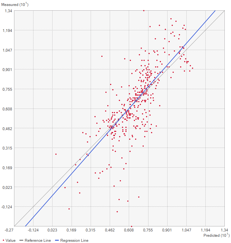
This method works by removing one of the points from the dataset and consequently interpolating the value for this point as if it was unknown. Repeating this for every single datapoint results in the mean error of the predictions. Graphing the measured value for each point against the predicted values results in a graph where under perfect conditions, the points should be on a perfect line. Since some errors are certainly made, the actual points are not along that line but a bit off. Creating a regression line, the error can be made visible by comparing the deviation of the regression line with the perfect 1:1 line.
Practical application of IDW
In this exercise, a point layer with temperature measurements spanning most of Europe as well as some neighboring regions is given. Based on a choice of AOI, the temperatures is interpolated for the whole AOI using the IDW method in ArcGIS Pro.
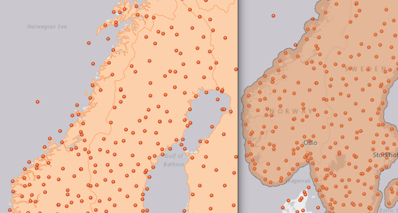
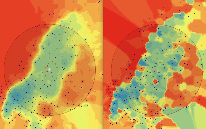
As the area of interest, the Fenoscandian nations of Sweden, Norway and Finland were chosen. Mainly because of their large north-south extent as well as the climate differences near the Atlantic cost compared to the near-continental climate of eastern Finland, quite large differences in temperature are to be expected. Additionally, in some areas the measurements are quite sparse, which might lead to the clearer manifestation of differences in IDW parameter settings.
Additionally, a 25 km buffer was drawn around the borders of the nations, since many measurement points are just outside of the vector boundary on small islands. Of course the IDW implementation in ArcGIS Pro creates the interpolation values and then clips the interpolated area to the boundary, but it is certainly of interest to enlarge the AOI a few km into the sea in order to visualize how the algorithm deals with the linear placement of the measurement points.
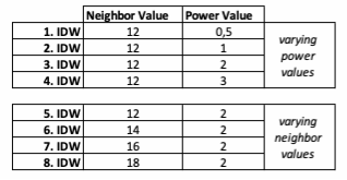
Based on the points and the boundary layer, the IDW was performed multiple times with changing parameters. The interpolation was performed 4 times with varying Neighbor and 4 times with varying Power parameters:
For the visualization, a single color ramp made out of shades of green was chosen. Multiple colors make it harder to visualize the continuety, since putting all colors on a scale of warmer to colder does not arrive naturally to every user. These shades of green seemed to be easily distinguishable as well as easing the comprehension that darker equals wormer. The classes were defined in 3° steps starting from 0 up to 15, which is just above the maximum value.
Regarding the Neighbors parameter, the differences between 12, 14, 16 and 18 are not very big. Apparently, extending the “radius” to more neighboring points does not change the resulting interpolated map on this scale. This is also confirmed by inspecting the histograms, which show very similar mean values and distributions.
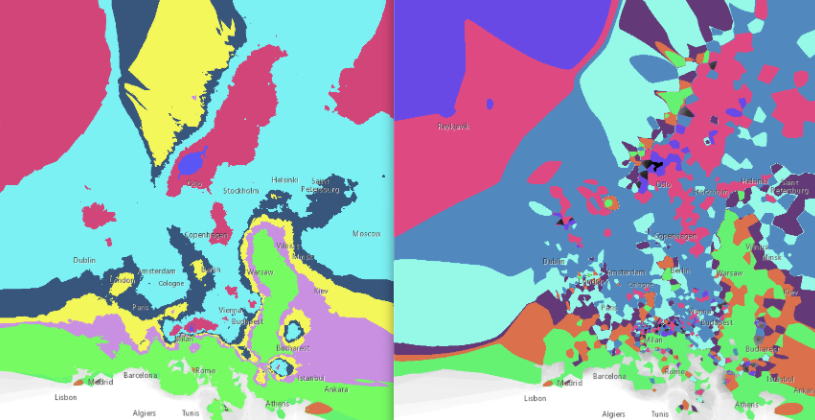
In this area of interest, changing the Power parameter on the other hand has a high influence the interpolation result. With a lower value, the areas exhibit a larger clustering and a larger spatial auto-correlation than with higher values (to test that claim, the Moran’s I value will also be calculated at the end of the exercise). Since raising the power value strengthens influence of spatially nearer known points, the map becomes much more fragmented. To visualize this phenomenon better, the Geospatial Wizard was used to quickly visualize the interpolation areas with extremely high and extremely low power.
IDW quality assessment of AOI
Now it is time to look at the quality assessment for our Area of Interest. Using the Geospatial Wizard and the above-described method, we look at the mean averages for our most extreme cases for the power parameter, since that shows the biggest difference.
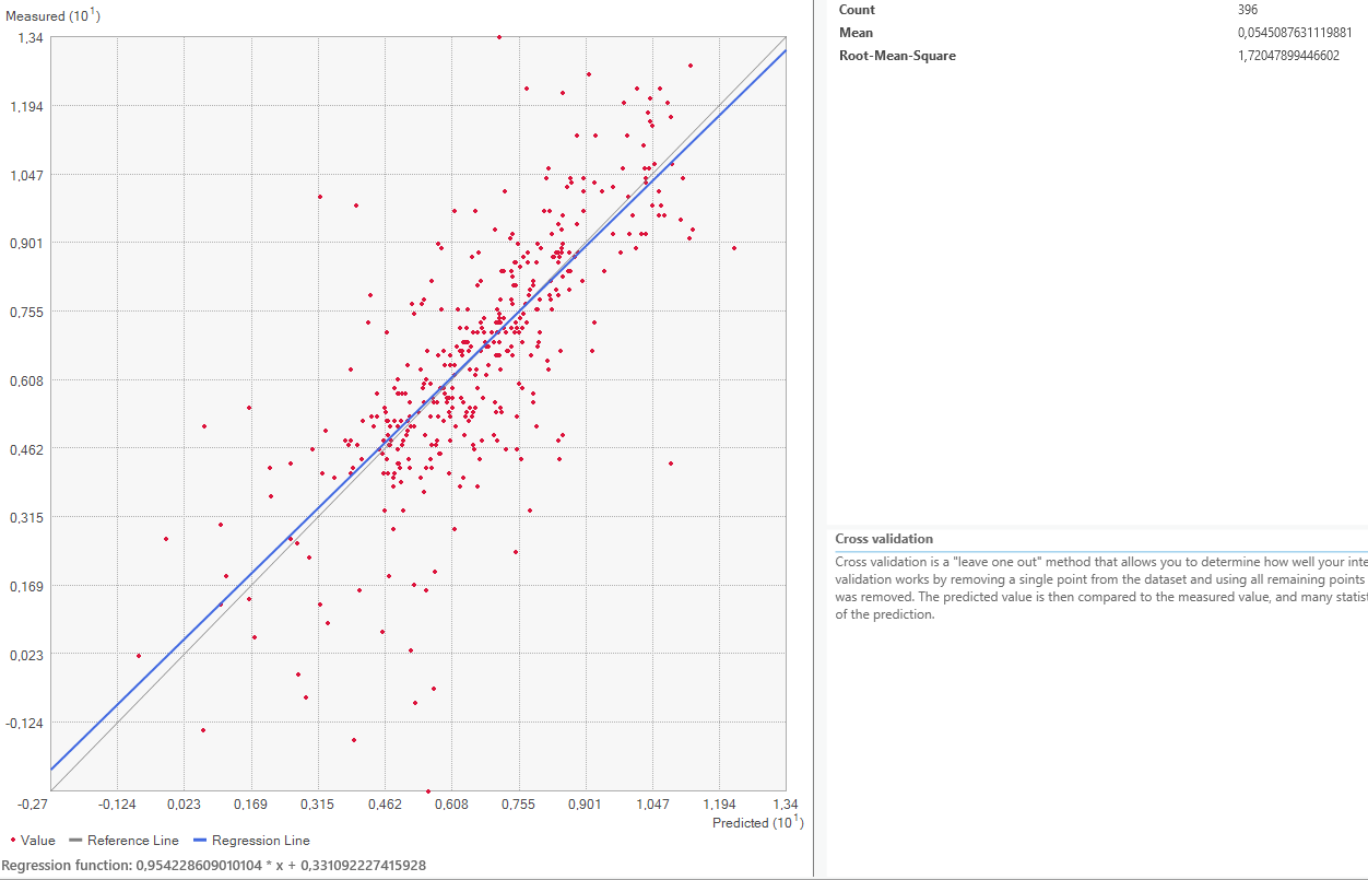
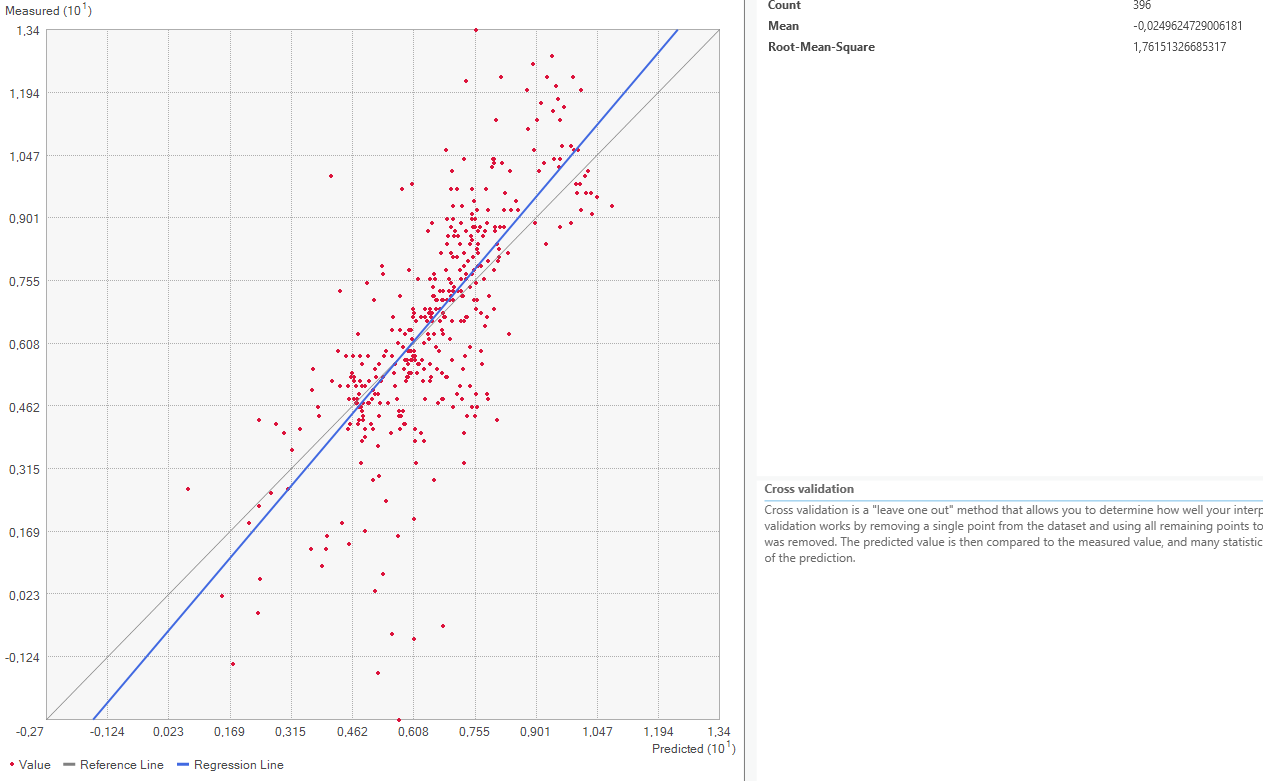
On closer inspection of the quality assesment methods, it is questionable how valid this method is. The regression line is closer to the expected line for the power 1 setting, but the mean error worse. This might be because both “upwards” and “downwards” errors are taken to calculate the mean value. Therefore, a higher standard deviation equally distributed both upwards and downwards might be evened out and lower error rate shown than is actually warranted.
Moran’s I applied to IDW results
Trying to verify the previous assumption that a higher power value more sharply fragments the result, the Moran’s I spatial auto-correlation values were calculated for the power parameters 1 and 20. Since I previously worked with this method and already created the code a while ago, it seems interesting to try it out on this dataset. Unfortunately, I was not able to draw any conclusions from this method. It returns a value very close to +1 for every tiff I throw at it, even ones where I would say the spatial autocorrelation should be lower, more towards 0 and thus “random” distribution. I would be happy to hear some feedback on the method, which is described in detail below.
Firstly, the raster images were reclassified.
The Moran’s I value is calculated with the following code, which also creates the charts:
The graphs and values returned from the method are as follows:
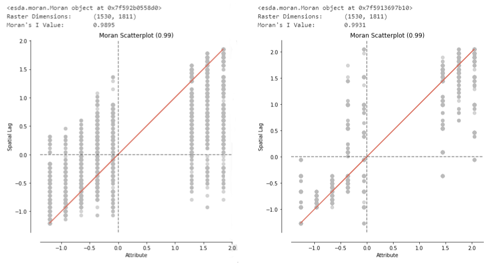
I am quite sure that the implementation of the Moran’s I algorithm works properly, as seen in my GitHub repository which runs the caculation on some sample images: