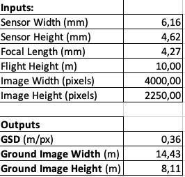
Ground Sampling Distance
The GSD shows the spatial resolution of the image on ground level. It is important not to fly too high in order to still be able to spot the GSDs and get high-enough resolution images, while flying too low limits the speed of acquisition and increases processing time.
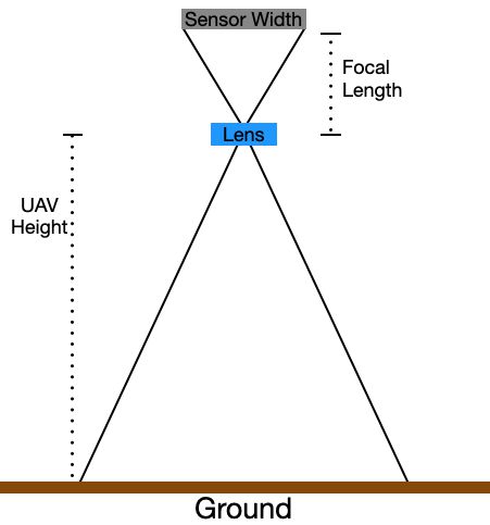
Input parameters are the Sensor Width in mm, the focal length in mm, the width of the image in pixels and the UAV height in m. My GSD calculation is inspired by this tutorial.
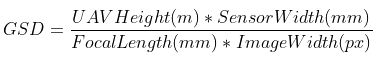
Solving the Formula for a height of 10m and the DJI Mavic Mini camera parameters results in a GSD of 0.36cm/pixel (mistyped in table 1 as 0.36m/pixel).
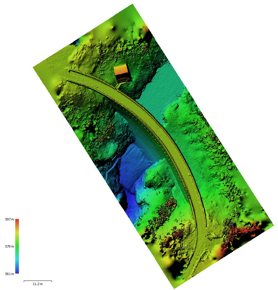
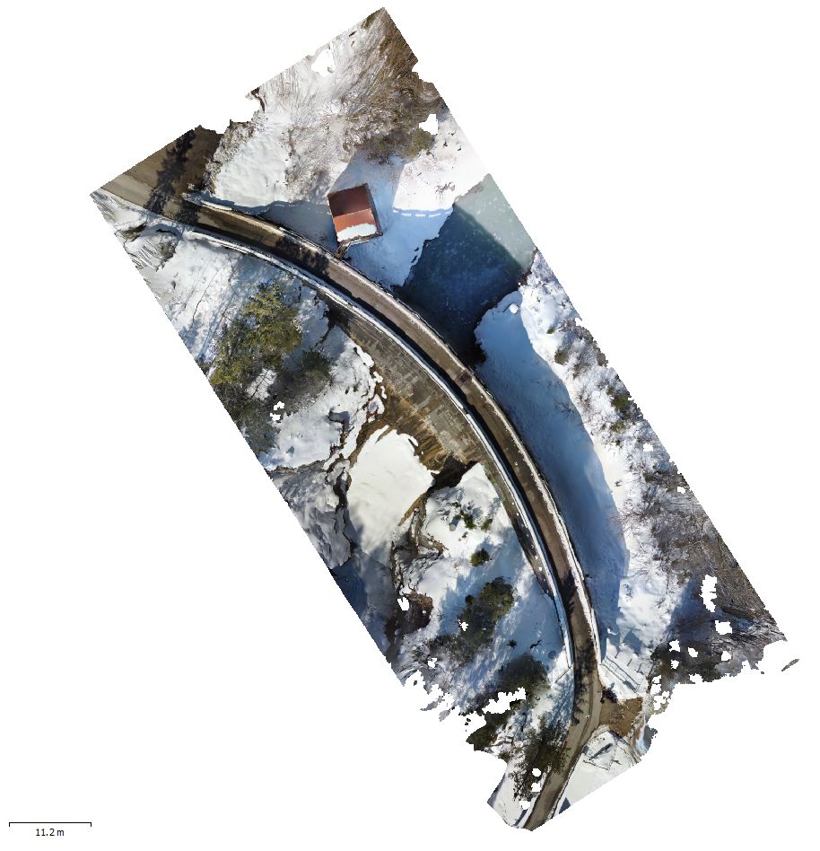
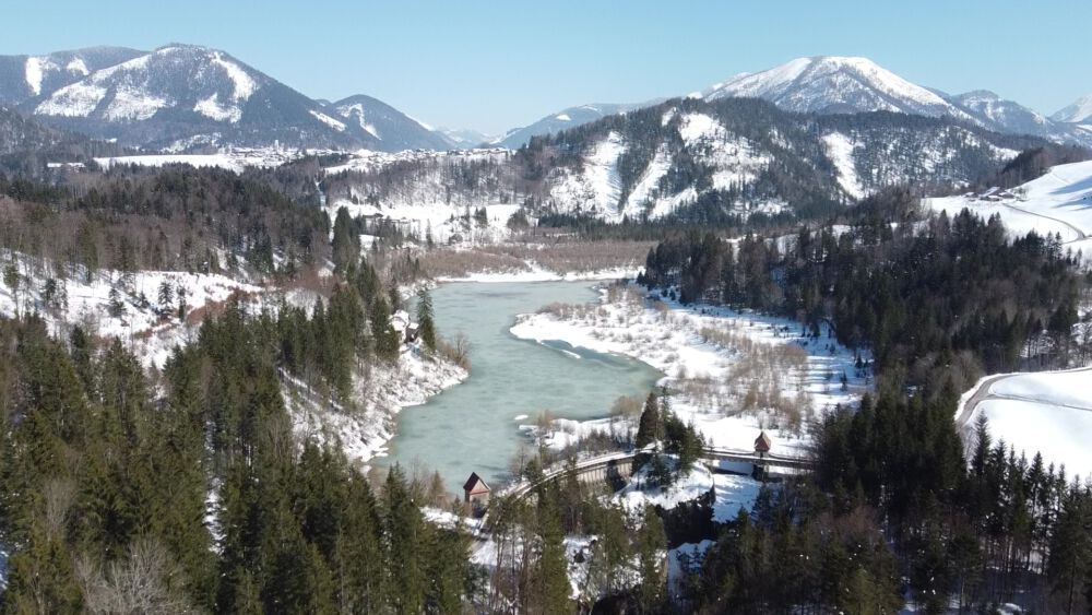
The main barrage of the dam is chosen as the object of interest, not the spillway to the south of the main complex. More specifically, the wall itself on both sides as well as the maintenance building to the north of the dam, including some adjacent rock/riverbed areas right next to the dam.
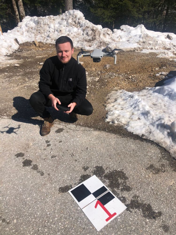
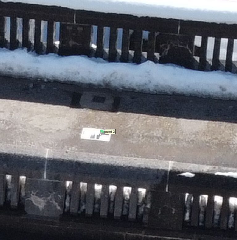
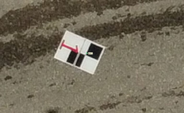
Three Ground Control Points (GCPs) were set up and their coordinates mapped. Thei height information was extracted by referencing the GCPs to a 1m DSM. The xyz coordinates were then saved as a .csv file. Unfortunately, a passing car promptly destroyed the third GCP, therefore only two were used during the process.
Mesh Creation
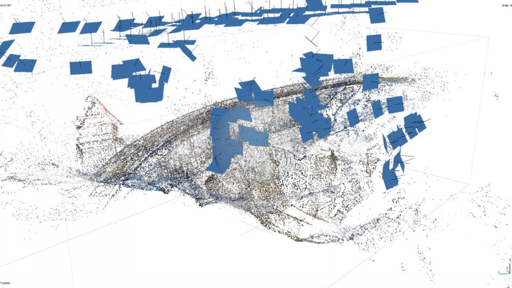
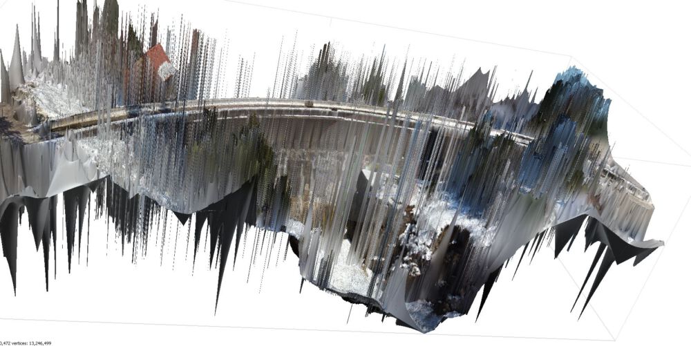
Consulting the documentation, based on these almost 200 images with 12mp each, over 400gb of RAM would be needed for the arbitrary (3D) mesh. The 2.5D height mesh requires 13gb, which is managable. An important issue seems to be the many small leaves and branches portruding from the trees into the “open”, creating many points with low spatial correlation, significantly increasing the RAM usage.
The 2.5D mesh could be sucessfully calculated, but of course projects the created faces on a 2D surface with height coordinates, making the mesh more or less useless.
The Dense Point Cloud was recalulated on ‘medium’ quality, resulting in a total of 8,000,000 points. From that, there is no issue calculating a 3D model with the ‘arbitrary’ settings.