Assessing Ship Sizes using SAR – Practical Application of Mathematic Morphology

Introduction

Based on the paper by M. Stasolla and H. Greidanus from 2016, a workflow is followed to estimate ship sizes based on Sentinel-1 imagery. Most importantly, a fundamental element in their workflow is the usage of mathematical morphology to “clean” the SAR image in order to estimate the real-world boundaries of ships.

Figure 1, original description from paper: Results of the various processing steps described in Section 2: (a) tgt; (b) tgt_HED; (c) tgt_ROT; (d) tgt_X; (e) tgt_Y; (f) tgt_XY; (g) tgt_XY_BW and (h) rectangle of derived length and width laid over the original amplitude image. The area of the frames is 200 m 200 m. In (a), (b) and (h), range is horizontal and azimuth is vertical. The pixel values of coloured images range from 0 (blue) to maximum (red); binary results are shown in black and white. The green rectangles in (a), (c) and (g) represent the minimum bounding box enclosing the pixel cluster.

The same methods will be adapted for a Sentinel-1 image from the entrance of the Suez Canal from the end of March 2021, showing a large accumulation of ships waiting for the obstruction of the canal to clear.

Data

The data used in this project is a Sentinel-1 SAR VV-polarized single band image from the 29th of March 2021, downloaded from Google Earth Engine.

Preprocessing for Morphology

First, a small subset of several ships es extracted, since a small image is easier to work with during the testing phase.

In order to prepare the data for the binary mathematical morphology, the values of the image are reclassified based on a threshold, which is manually chosen. The threshold chosen is 0, being the divider between negative values (bo reflectance to sensor) and positive values (where a return is measured). The resulting image still has some error pixels and the ships are quite deformed.

Workflow

As outlined in the paper, the workflow starts with a multi-angular erosion, followed by a thresholding for their specific purpose. Following a rotation, multi-scale openings and closings are performed, which are then added. The final result, after another thresholding, is a minimum bounding box of the ship.

The workflow relies heavily on a thresholding via CFAR, after some testing it becomes clear that the implementation unfortunately exceeds the scope of this exercise. Since the paper mentions some alternatives to CFAR, namely Otsu’s thresholding method, this was implemented instead.

Notebook

This Jupyter Notebook recreates the workflow of the paper on a subset test image than the original Suez Canal image. As outlined in the notebook, compromises needed to be made with regards to certain steps since they were not reproducible. Additionally, some thresholds that were calculated adaptively in the paper were selected manually. At the end, a ship mask is still obtained.

The data and all notebooks, including the notebook on the full dataset, can be found on GitHub.

workflow_test_data

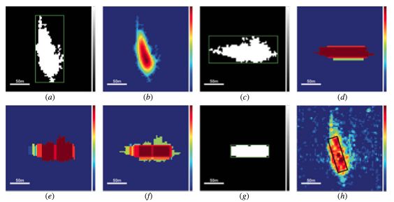
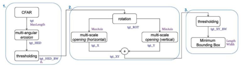
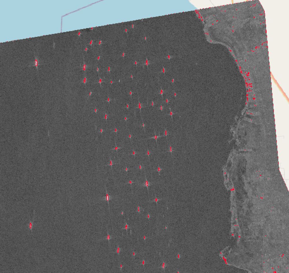
Implementing Workflow¶

Paper: https://www.tandfonline.com/doi/full/10.1080/2150704X.2016.1226522
Workflow:

T.o.C.:

Preparation 0.1 Loading Data 0.2 Defining thresholding and plot functions
Step 1: 1.1 Thresholding 1.2 Multi-Angular erosion 1.3 Thresholding
Step 2: 2.1 Rotation 2.2 Multi-Scale Opening 2.3 Addition of results
Step 3: 3.1 Thresolding 3.2 Minimim Bounding Boxes
Export Results 4.1 Create Ship mask 4.2 Write Ship Mask to Band

0. Preparation¶

0.1 Loading Data¶

In [2]:

import scipy.ndimage
import rasterio
import skimage.morphology
from matplotlib import pyplot as plt
import matplotlib
import numpy as np
import random
import matplotlib.pyplot as plt
from skimage import data
from skimage.filters import threshold_otsu
from numpy.ma import masked_array
import numpy.ma

from skimage.morphology import (erosion, dilation, opening, closing, white_tophat)
from skimage.morphology import black_tophat, skeletonize, convex_hull_image  # noqa
from skimage.morphology import disk
import numpy as np
import numpy.ma as ma

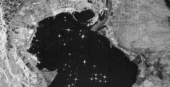
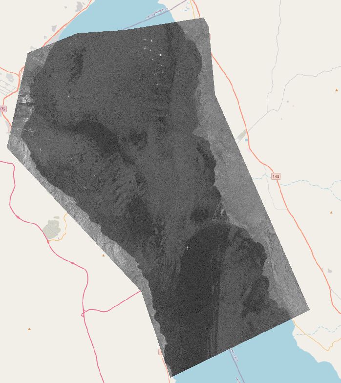
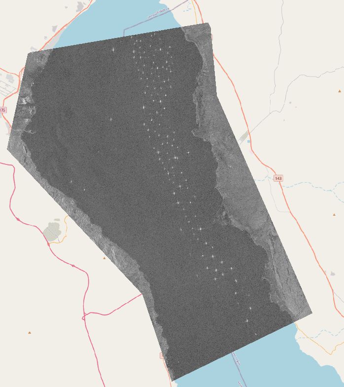
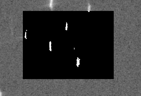
input_file_path = "data/test_data_crop.tif"

In [ ]:

In [3]:

# Read image and raster
src = rasterio.open(input_file_path)
array = src.read(1)

plt.imshow(array,cmap="gray")

Out[3]:

<matplotlib.image.AxesImage at 0x7efdea067490>

0.2 Defining thresholding and plot functions¶

In [4]:

def plot_comparison(original, filtered, filter_name):

    fig, (ax1, ax2) = plt.subplots(ncols=2, figsize=(15, 10), sharex=True,
                                   sharey=True)
    ax1.imshow(original, cmap=plt.cm.gray)
    ax1.set_title('original')
    ax1.axis('off')
    ax2.imshow(filtered, cmap=plt.cm.gray)
    ax2.set_title(filter_name)
    ax2.axis('off')

In [5]:

def otsu(array,plot):
    image = array
    thresh = threshold_otsu(image)
    binary = image > thresh
    
    
    if plot:
        image_masked = np.multiply(image,binary)
        fig, axes = plt.subplots(ncols=3, figsize=(15, 4))
        ax = axes.ravel()
        ax[0] = plt.subplot(1, 3, 1)
        ax[1] = plt.subplot(1, 3, 2)
        ax[2] = plt.subplot(1, 3, 3, sharex=ax[0], sharey=ax[0])

        ax[0].imshow(image, cmap=plt.cm.gray)
        ax[0].set_title('Original')
        ax[0].axis('off')

        ax[1].hist(image.ravel(), bins=256)
        ax[1].set_title('Histogram')
        ax[1].axvline(thresh, color='r')

        ax[2].imshow(binary, cmap=plt.cm.gray)
        ax[2].set_title('Thresholded Mask')
        ax[2].axis('off')

        plt.show()
    
    #return image values only for True pixels
    return(binary)

In [6]:

# test functions
plot_comparison(array, np.multiply(array,otsu(array,True)), "thresholded")

1. Step 1¶

1.1 Thresholding¶

In [7]:

mask_step_1 = otsu(array,False)
image_masked_step_1 = np.multiply(array,mask_step_1)

1.2 Multi-Angular Erosion¶

Instead of 5° steps, 4 steps of 45° are implemented. (Note: how to get 5° slope in np?)

In [8]:

plot_comparison(array,erosion(image_masked_step_1,skimage.morphology.rectangle(10,5)),"Erosion Rectangle")

In [9]:

se_1 = np.array([[0,0,0,0,0,1,0,0,0,0],
                [0,0,0,0,0,1,0,0,0,0],
                [0,0,0,0,0,1,0,0,0,0],
                [0,0,0,0,0,1,0,0,0,0],
                [0,0,0,0,0,1,0,0,0,0],
                [0,0,0,0,0,1,0,0,0,0],
                [0,0,0,0,0,1,0,0,0,0],
                [0,0,0,0,0,1,0,0,0,0],
                [0,0,0,0,0,1,0,0,0,0],
                [0,0,0,0,0,1,0,0,0,0],
                ])

se_2 = np.array([[1,0,0,0,0,0,0,0,0,0],
                [0,1,0,0,0,0,0,0,0,0],
                [0,0,1,0,0,0,0,0,0,0],
                [0,0,0,1,0,0,0,0,0,0],
                [0,0,0,0,1,0,0,0,0,0],
                [0,0,0,0,0,1,0,0,0,0],
                [0,0,0,0,0,0,1,0,0,0],
                [0,0,0,0,0,0,0,1,0,0],
                [0,0,0,0,0,0,0,0,1,0],
                [0,0,0,0,0,0,0,0,0,1],
                ])

se_3 = np.array([[0,0,0,0,0,0,0,0,0,0],
                [0,0,0,0,0,0,0,0,0,0],
                [0,0,0,0,0,0,0,0,0,0],
                [0,0,0,0,0,0,0,0,0,0],
                [0,0,0,0,0,0,0,0,0,0],
                [1,1,1,1,1,1,1,1,1,1],
                [0,0,0,0,0,0,0,0,0,0],
                [0,0,0,0,0,0,0,0,0,0],
                [0,0,0,0,0,0,0,0,0,0],
                [0,0,0,0,0,0,0,0,0,0],
                ])

se_4 = np.array([[0,0,0,0,0,0,0,0,0,1],
                [0,0,0,0,0,0,0,0,1,0],
                [0,0,0,0,0,0,0,1,0,0],
                [0,0,0,0,0,0,1,0,0,0],
                [0,0,0,0,0,1,0,0,0,0],
                [0,0,0,0,1,0,0,0,0,0],
                [0,0,0,1,0,0,0,0,0,0],
                [0,0,1,0,0,0,0,0,0,0],
                [0,1,0,0,0,0,0,0,0,0],
                [1,0,0,0,0,0,0,0,0,0],
                ])
se_multiangle = [se_1,se_2,se_3,se_4]

In [10]:

for se,degree in zip(se_multiangle,["90°","45°","0°","135°"]):
    plot_comparison(image_masked_step_1,erosion(image_masked_step_1,se),"10px flat Erosion at "+degree)