In [1]:
from skimage import color
from skimage import io
import numpy as np
import matplotlib.pyplot as plt
import cv2
In [2]:
#function to convertrgb to gray
def to_gray(img_rgb):
    red = img_rgb[:,:,0]
    green = img_rgb[:,:,1]
    blue = img_rgb[:,:,2]
    gray = 0.298*red + 0.587*green + 0.114*blue
    return(gray)
In [3]:
dolphins = plt.imread("dolphins.jpg")
dolphins_gray = to_gray(dolphins)

plt.imshow(dolphins_gray,cmap="gray")
plt.show()

2.2 Apply Transformations
In [4]:
# playing around woth classes
class image_transformer:
    def __init__(self,img):
        # get image parameters
        self.img = img
        self.h = img.shape[0]
        self.w = img.shape[1]
        self.dim = (self.w,self.h)

    def rotate(self,angle):
        #implement
        affine_matrix = (np.array([
            [np.cos(angle),-np.sin(angle),0],
            [np.sin(angle), np.cos(angle),0]]))
        return_img = cv2.warpAffine(self.img,affine_matrix,self.dim)
        return(return_img)

    def scale(self,factor):
        factor = float(factor) # to prevent CV error
        affine_matrix = np.array([
            [factor,0,0],
            [0,factor,0]])
        return_img = cv2.warpAffine(self.img,affine_matrix,self.dim)
        return(return_img)

    def translate(self,x,y):
        x = float(x)
        y = float(y)
        affine_matrix = np.array([
            [1,0,x],
            [0,1,y]])
        return_img = cv2.warpAffine(self.img, affine_matrix, self.dim)
        return(return_img)

    def shear(self,s,x):
        s = float(s)
        x = float(x)
        affine_matrix = np.array([
            [s,x,0],
            [0,s,0]])
        return_img = cv2.warpAffine(self.img, affine_matrix, self.dim)
        return(return_img)


img_trans = image_transformer(dolphins)
In [5]:
plt.figure(figsize=(10,8))
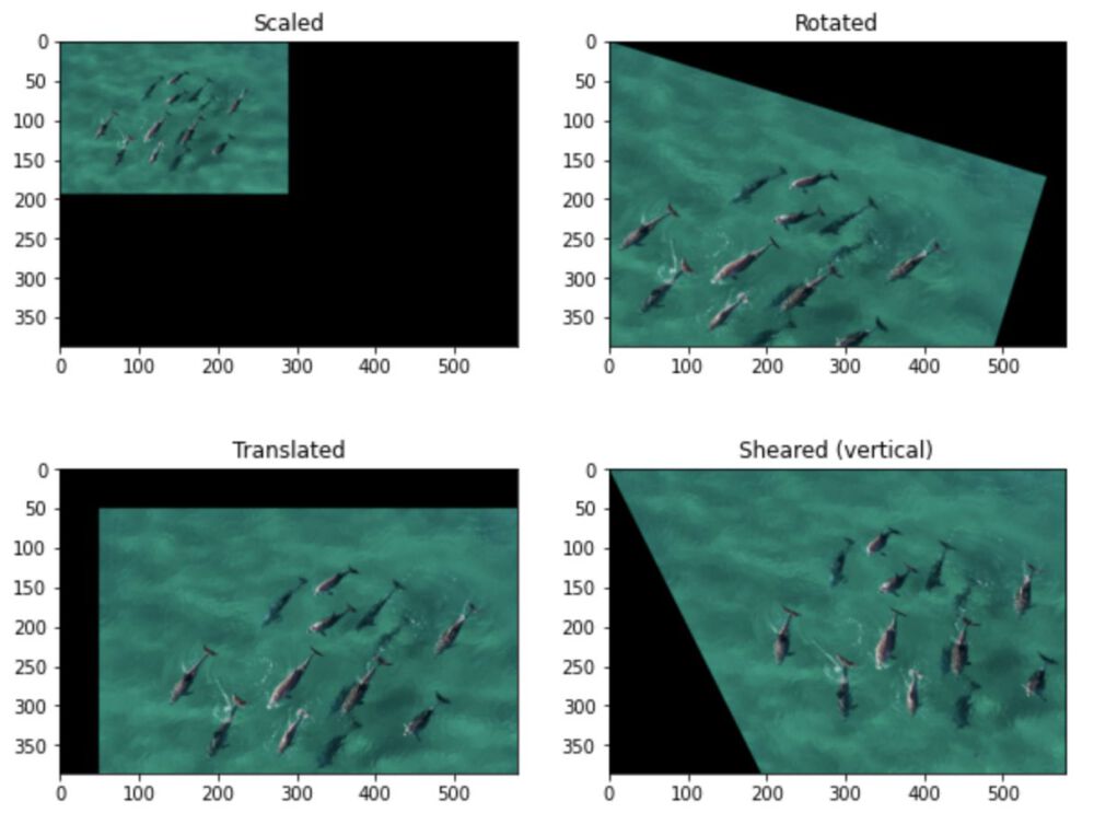
plt.subplot(2,2,1)
plt.imshow(img_trans.scale(0.5))
plt.title("Scaled")
plt.subplot(2,2,2)
plt.imshow(img_trans.rotate(0.3))
plt.title("Rotated")
plt.subplot(2,2,3)
plt.imshow(img_trans.translate(50,50))
plt.title("Translated")
plt.subplot(2,2,4)
plt.imshow(img_trans.shear(1,0.5))
plt.title("Sheared (vertical)")
plt.show()

2.3 NN vs. Bilinear vs Bicubic Interpolation
In [7]:
# Downsize original to see differences


scale_percent = 20
width_small = int(dolphins.shape[1] * scale_percent / 100)
height_small = int(dolphins.shape[0] * scale_percent / 100)
dim = (width_small, height_small)
img_small = cv2.resize(dolphins,dim)
In [9]:
# upsampling back to original size
img_nn  = cv2.resize(img_small, (dolphins.shape[1],dolphins.shape[0]) , interpolation = cv2.INTER_NEAREST)
img_bil = cv2.resize(img_small, (dolphins.shape[1],dolphins.shape[0]), interpolation = cv2.INTER_LINEAR)
img_bic = cv2.resize(img_small, (dolphins.shape[1],dolphins.shape[0]), interpolation = cv2.INTER_CUBIC)


plt.figure(figsize=(14,10))
plt.subplot(2,2,1)
plt.imshow(img_small)
plt.title('Downsampled')
plt.subplot(2,2,2)
plt.imshow(img_nn)
plt.title('Nearest Neighbor')
plt.subplot(2,2,3)
plt.imshow(img_bil)
plt.title('Bilinear')
plt.subplot(2,2,4)
plt.imshow(img_bic)
plt.title('Bicubic')
plt.show()

- Nearest Neighbor just upsamples the image without any modification, assigning an area of the scale factor a single value. The optical impression of the image does not change.
- The bilinear method creates an average over the connections of the pixel, with the newly created pixel being assigned the average of the sourrounding pixels. This metod helps tocreate a better visual effect, but also might introduce artifacts and noise to the data.
- Bicubic interpolation is smoother, because instead of linear straight-line connections between neighboring pixel-values curves are used. This uses a larger neighborhood/matrix of pixel to determine the newly assigned value, weighting the influence by the distance.
In [10]:
dolphins_lab = cv2.cvtColor(dolphins,cv2.COLOR_BGR2Lab)

plt.figure(figsize=(14,10))
plt.subplot(2,2,1)
plt.imshow(dolphins_lab)
plt.title('Original Image (LAB) visualized in RGB space')

plt.subplot(2,2,2)
plt.imshow(dolphins_lab[:,:,0],cmap="gray")
plt.title('L')

plt.subplot(2,2,3)
plt.imshow(dolphins_lab[:,:,1],cmap="gray")
plt.title('A')

plt.subplot(2,2,4)
plt.imshow(dolphins_lab[:,:,2],cmap="gray")
plt.title('B')
plt.show()

In [11]:
dolphins_hls = cv2.cvtColor(dolphins,cv2.COLOR_BGR2HLS)

plt.figure(figsize=(14,10))
plt.subplot(2,2,1)
plt.imshow(dolphins_hls)
plt.title('Original Image (HLS) visualized in RGB space')

plt.subplot(2,2,2)
plt.imshow(dolphins_hls[:,:,0],cmap="gray")
plt.title('H')

plt.subplot(2,2,3)
plt.imshow(dolphins_hls[:,:,1],cmap="gray")
plt.title('L')

plt.subplot(2,2,4)
plt.imshow(dolphins_hls[:,:,2],cmap="gray")
plt.title('S')
plt.show()

HSL - (Hue Saturation, Lightness)
3.2 Thresolding by Color of Interest
In [12]:
plt.figure(figsize=(20,20))

for count,(i,sp) in enumerate(zip([dolphins[:,:,0],dolphins[:,:,1],dolphins[:,:,2]],[321,323,325])):


    # histogram
    plt.subplot(sp)
    histogram,bins = np.histogram(i,99999)
    plt.plot(bins[:-1],histogram)
    plt.title("Histogram Channel "+str(count))

    # image
    plt.subplot(sp+1)
    plt.imshow(i,cmap="viridis")
    plt.title("Image Channel "+str(count))

plt.show()

The Histograms can tell which pixel values correspond to the area of interest, in this case the dolphins. The only bright areas in the R channel (whiter areas in the RGB) seem to be a good separator, additionally the other chanels whould be quite high aswell, but surely over the histogram peak caused by the blue-ish ocean.
In [13]:
def rgb_thresholding(img,R,G,B):

    # define subfunction checking if values are in range
    def check_condition(px,R,G,B):
        if px[0]>R[0] and px[0]<R[1] and px[1]>G[0] and px[1]<G[1] and px[2]>B[0] and px[2]<B[1]:
            return(1)
        else:
            return(0)

    img_ls = []
    for row in img:
        row_ls = []
        for pixel in row:
            # perform check, write to new array
            row_ls.append(check_condition(pixel,R,B,G))

        # append row to total list
        img_ls.append(row_ls)

    # return binary mask for condition
    return(np.array(img_ls))
In [14]:
# optimizing for surfaced amnimals, not submerged ones
dolphin_mask = rgb_thresholding(dolphins,R=(30,255+1),B=(0,150),G=(0,120))

plt.figure(figsize=(10,10))
plt.subplot(2,1,1)
plt.imshow(dolphins)
plt.title('Original Dolphin Image')

plt.subplot(2,1,2)
plt.imshow(dolphin_mask,cmap="gray")
plt.title('Dolphin Mask')
plt.show()

Fidning a clear separation for this image was not easy doe to the similar color tones and the half-submerged state of some of the animals, but the result is still very close to the visual observation.
In [ ]: