Radar Assignment
For this assignment, the steps of the given tutorial are followed and protocolled. Screenshots with descriptions are inserted to show the progress and the Questions answered in the order that the time they are posed.
The study area is in the Andalusia region of Spain, where a wildfire occurred in the summer of 2017. The images in question are Sentinel-1 radar images from the 02.07.2017 and the 19.08.2017, before and after the event in question. Using SNAP, the images are cropped, orbit corrected, calibrated, coregistered, a change detection performed, geometrically corrected and finally filtered for speckles. The final output is exported and visualized, as well as compared to the information provided by the Copernicus Emergency Management Service for this particular event. At the end of the assignment, hopefully we will have learned all the reasons why these particular steps are performed and get familiar with the terminology and processes of radar image analysis.
Question 1: Metadata
S1B_IW_GRDH_1SDV_20170702T062605_20170702T062630_006305_00B160_6DA0
Flight Direction: Descending
Polarizations: VH + VV
S1B_IW_GRDH_1SDV_20170819T062608_20170819T062633_007005_00C576_066C
Flight Direction: Descending
Polarization: VH + VV
Question 2: Polarization
The letters V and H stand for polarization directions, meaning horizontally and vertically. Polarization itself describes the axis of oscillation along the path of the signal. Since the properties of the reflecting object can change this axis, it is of interest to see if the polarization of a known signal is changed during the reflection process.
The order in which the polarizations are given shows the emission and reception of the signal, so for VH it means the signal is sent in a vertical polarization but the filter in front of the sensor only lets the horizontally polarized signal through.
VH: Vertical pol. emission, horizontal pol. reception
VV: Both vertical pol. emission and reception
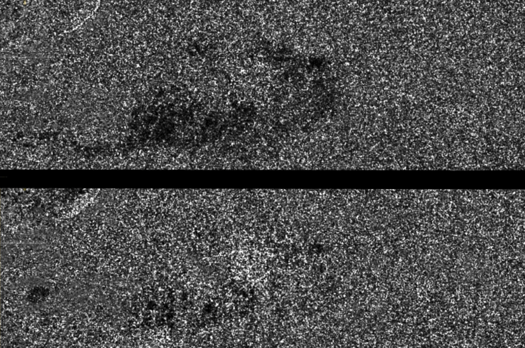
Question 3: Intensity & Amplitude
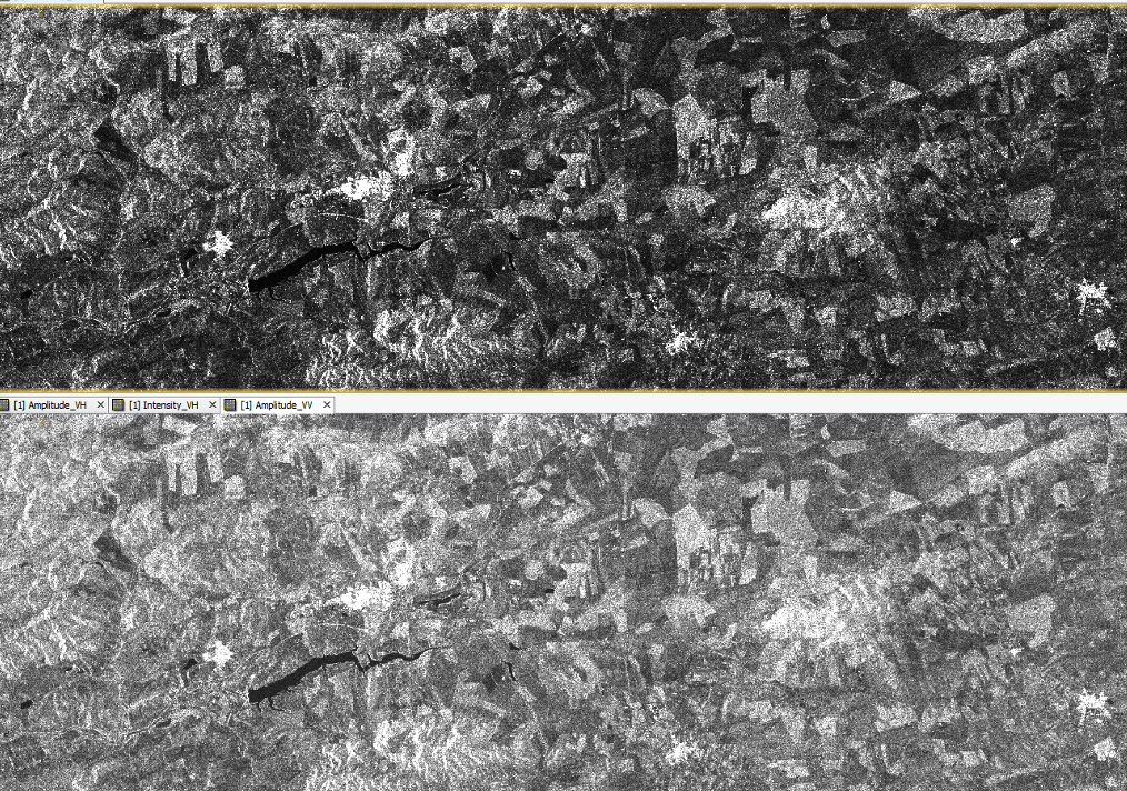
For each polarization, both an amplitude and intensity band are available. The polarizations only describe the axis of oscillation of the wave, meaning the bands are differentiated between by the way of reflectance. Amplitude is the measurement of the strength of a signal as measured by the sensor itself, referring to the amount of energy transmitted. The intensity is the amplitude squared, which explains the higher values and thus the different appearance or the image above. The intensity image is used for calibration and classification of features, since the intensity is more representative of surface properties.
Question 4: Comparison of different Land Use Areas
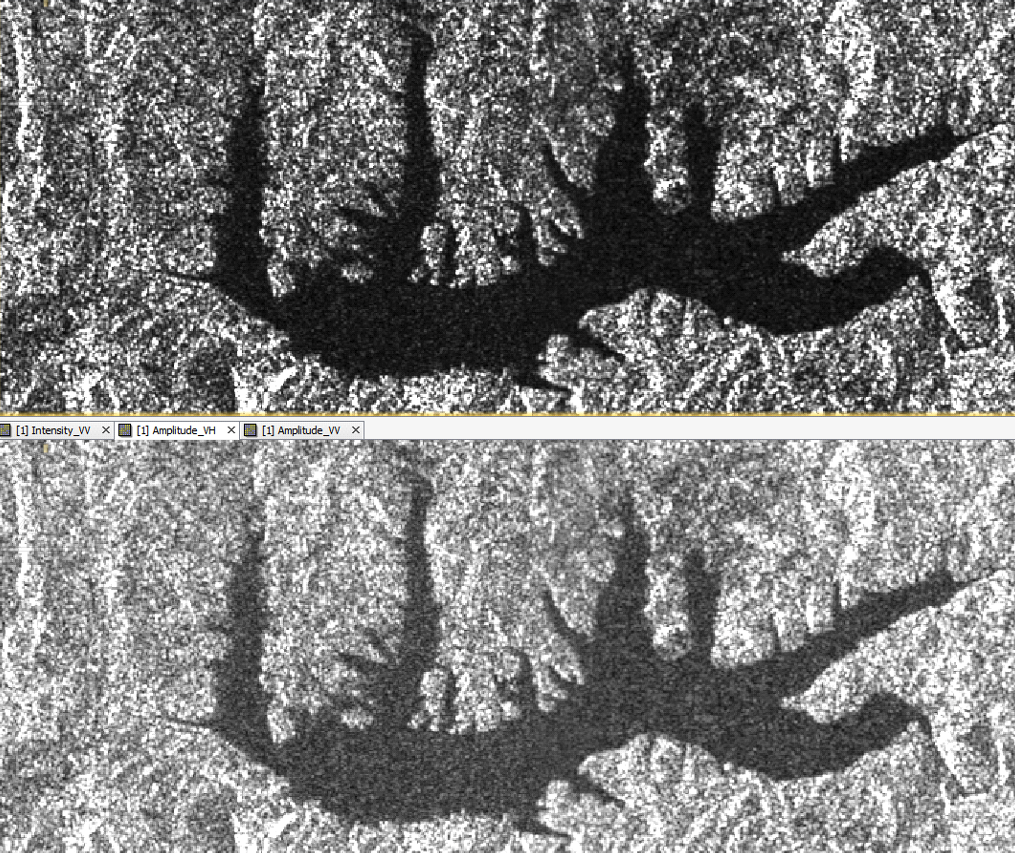
The VH image appears much less “grainy” or “speckled”. The body of water seems to reflect the signal much more like a mirror (angle of incidence == angle of reflection) in the VH image, since the pixels appear darker. The same effect is visible on the surrounding area, with the vegetation showing a darker level in general than in the VV image.
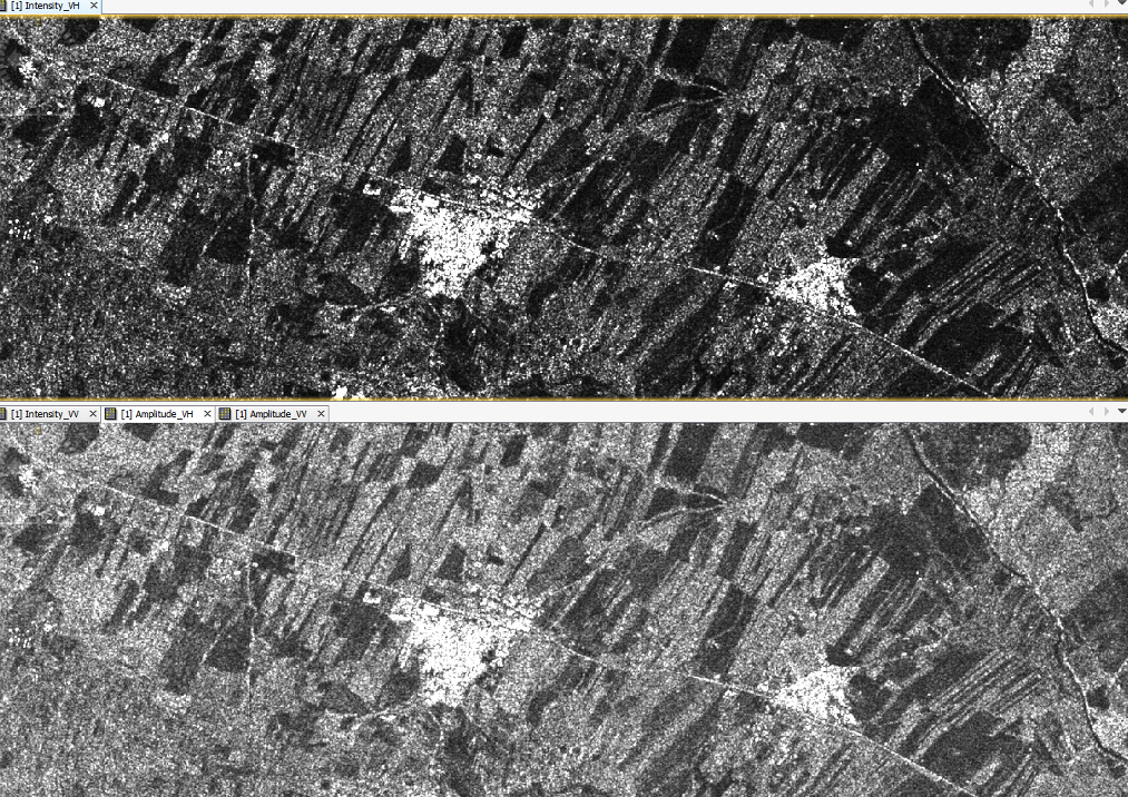
The general observations of the lake and scrublands image hold true also for this area of interest. In this case however, the VV image seems more suitable in differentiating between different fields and therefore possibly different crops. On the other hand, the VH image shows more detail in the urban area since more roads and possibly even buildings are distinguishable.
Question 5: Orbit file correction
Applying the orbit file correction is necessary, because SAR orbit vectors are not necessarily very accurate by themselves. Since many sensors measure the exact orbit of the satellite, such as internal Gyros, GPS and ground-based observation methods, the exact orbit and/or position of the satellite needs to be calculated after the image was taken. The satellite images don’t come with all this information included, so in order to archive a higher accuracy all the positioning sensor data is combined in SNAP to give the best accuracy and therefore improve geocoding/georeferencing.
Since the orbit correction does not alter the appearance of the image but instead improves the geometric accuracy, no screenshot of the product is shown.
Question 6: sigma0, gamma0 and beta0
For this application, we are most interested in the sigma0 band, because this band represents the backscatter information returned to the sensors from objects on the ground. The reflection values of the image are mathematically normalized and therefore called “backscatter coefficient”. This information in particular is reflective of surface parameters such as surface roughness, geometric shape and dielectric (electrical insulation) properties of the surface.
The Beta0 and Gamma0 bands contain different information. The Beta0 band is the radar brightness coefficient, which the ESA defines as the “reflectivity per unit area in slant range which is dimensionless”. Gamma0 on the other hand is a measurement of the absolute radar energy emitted and received by the satellite.
Next, an image coregistration is performed which combines the different bands of the images into one image, leading to the effect that the different information is presented on the screen via different RBG bands.
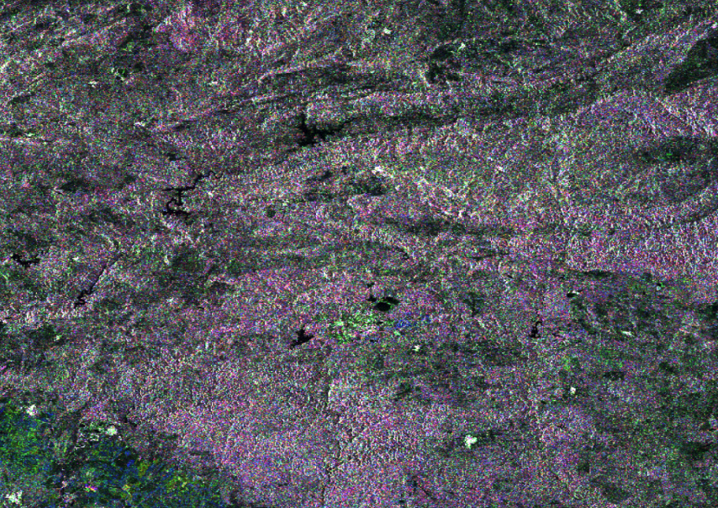
Question 7: Change Detection Comparison
This image shows the VH and VV polarization change detection results, where a clear visually darker area can be seen in the VH polarization image. The other polarization also has an area of conformity, but this is much less clearly distinguishable and leans towards a higher reflectance value and thus more towards a white color.
After this, the Range-Doppler Terrain orthorectification method offered by SNAP is used. This is necessary because due to the topography of the area of interest and the tilt of the sensor, pixels might not appear on their proper orthorectified positions. Common artifacts are foreshortening, layover and shadow. Only if the topography of the area is known, the shadows can be calculated and properly masked, as well as the pixels shifted to their correct positions in hilly areas. The Range-Doppler Terrain correction methods performs all these steps with the help of a DEM (Digital Elevation Model).
Finally, the grainy artifacts known as speckles are filtered. The noise is filtered by calculating a standard deviation of the pixel values and therefore filtering outliers. The final result appears a lot cleaner and easily understandable.
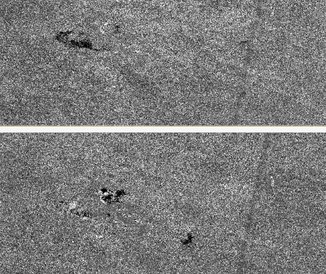
Figure 7 shows the final result after performing all steps in SNAP. This image is now exported as .tiff and loaded in QGIS. In order to be properly displayed, we need to look at the pixel value histogram of the image and map the 256 value color information in a meaningful way, so that we can distinguish between features in the image. By using the min-max setting and manually changing the range starting at 2% all the way to 98%, the image is properly visualized.
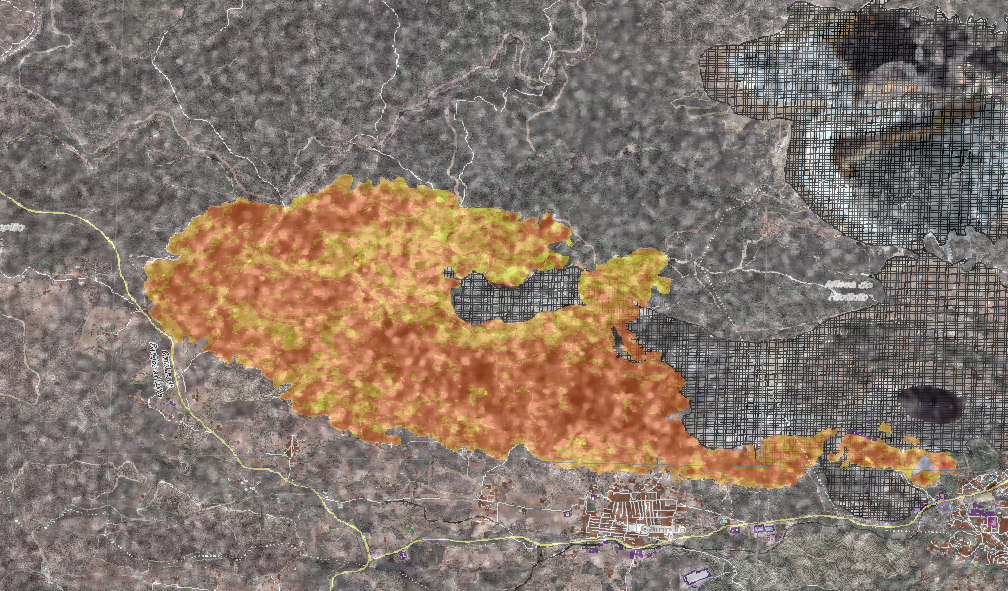
Question 8: Copernicus EMS – Evaluation
Then, a map is created in QGIS showing a side-by-side comparison for the VH and VV polarizations as well as the .tiff map produced by the EMS.
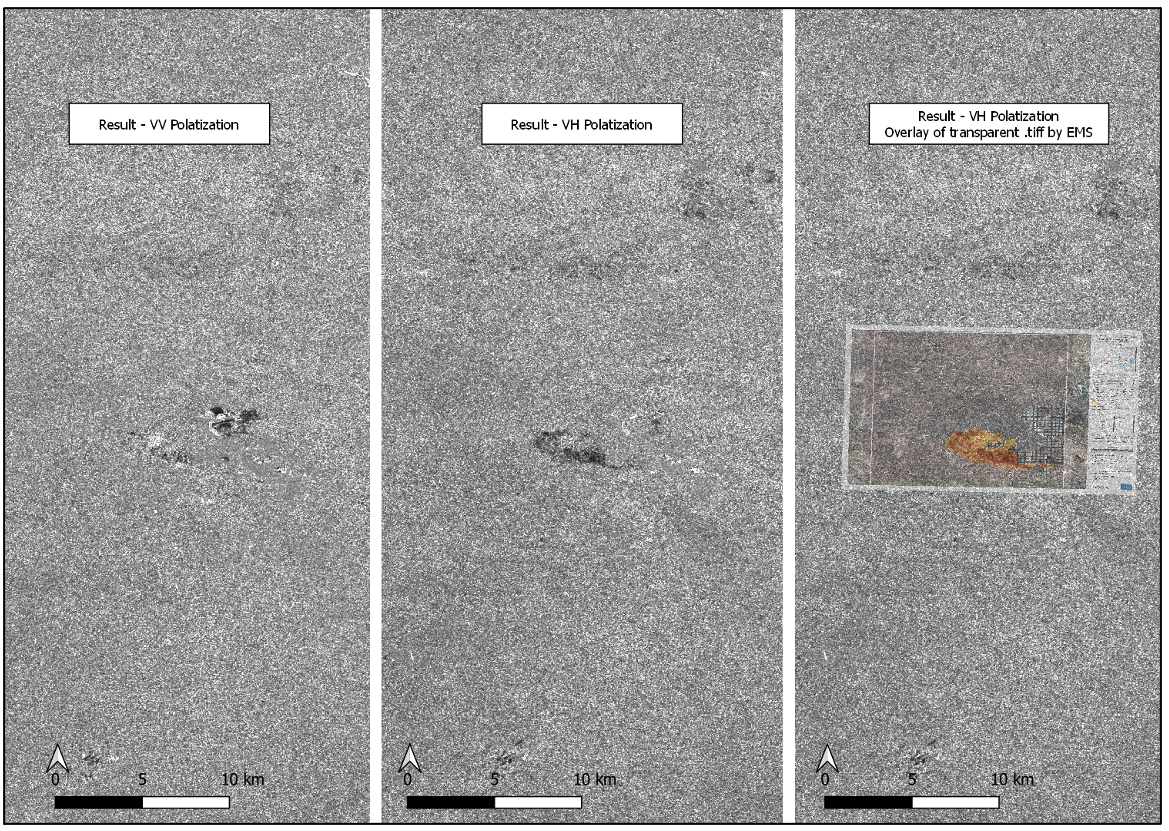
Dark areas are visible in both resulting images created by this tutorial. The VH polarization produces a clearer distinguishable burnt area than the VV polarization image, while the VV image also shows darker areas of conformity in the north-west of the burnt area. Looking at the burn extent as provided by the EMS, we can see that their classification of the burnt area aligns much better and clearer with the VH polarization result of this tutorial. Therefore, I conclude that the VH result is more suitable for detecting burnt areas than the VV image.
The main outcome/characteristic of the VV image is the clear visibility of the mine area. Looking at the area classified as “Industry/Utilities – Extraction Mine”, it lines up very well with the darker circular areas visible in the VV image.
Also, the orthorectifying and geocorrection have succeeded, since the areas align perfectly with the result provided by the EMS as well as the burnt area shapefile.
Conclusion
In retrospect, it can be said that we performed an analysis from the start to the finish. Starting from bare radar images, we performed and learned about all steps necessary to extract information from the data. By describing the tools and methods we used, insights into the inner workings of preprocessing radar data as well as the basics of radar technology and the geocorrection of images were gained.
It was also very interesting to see that both polarizations showed different results, with VH showing the mining area, while VV showed the burnt area. It was also reaffirming to see that a reputable source such as the EMS came to the same results, allowing us to retrace their steps and see that the techniques we learn about and use are also applied by organizations on the cutting edge of scientific applications.
This data needs to go through quite an extensive preprocessing scheme, which most likely is similar for many different applications. Steps such as the correction, speckle/noise reduction and the terrain correction surely are done by many researchers on their own time and machines; this might be a case for ARD (analysis ready data). Hosting preprocessed images might make radar data more accessible to a broader audience and save time for the end users.