Practical Lab: Linear Regression by using the gradient descent algorithm
Utilities
from sklearn import datasets # donnees
import os # rep de travail
import pandas as pd # data analysis
from scipy import stats # stat desc
import matplotlib.pyplot as plt # graphiques
import numpy as np # maths
import seaborn as sns
from sklearn.metrics import mean_squared_error, r2_score
from IPython.display import display, Image
Data
#-- Reading the (training) data in a data frame
df = pd.read_csv("pm25_train_data.csv",delimiter=";")
df.dropna(inplace=True)
df.head()
| PM2.5 | SO2 | NO2 | CO | O3 | temperature | pressure | dew point | rainfall | windspeed | |
|---|---|---|---|---|---|---|---|---|---|---|
| 0 | 24.0 | 7.0 | 13.0 | 300.0 | 74.0 | 3.9 | 1027.3 | -19.7 | 0.0 | 5.1 |
| 1 | 93.0 | 25.0 | 76.0 | 900.0 | 22.0 | 2.7 | 1027.3 | -16.4 | 0.0 | 2.7 |
| 2 | 117.0 | 77.0 | 99.0 | 1600.0 | 14.0 | 13.8 | 1012.5 | -13.3 | 0.0 | 1.1 |
| 3 | 58.0 | 12.0 | 14.0 | 400.0 | 77.0 | 14.2 | 1018.9 | -13.9 | 0.0 | 2.7 |
| 4 | 226.0 | 104.0 | 136.0 | 2299.0 | 15.0 | 11.9 | 1009.7 | -7.5 | 0.0 | 1.3 |
#-- Save the explanatory variables in a variable X (and their names in a varaible feature_names), and the target variable in Y
feature_names = list(df.columns[1:])
print("Feature Names: ",feature_names)

# extract target
Y = np.array(df["PM2.5"])

# extract variables
X = np.array(df[feature_names])
Feature Names: ['SO2', 'NO2', 'CO', 'O3', 'temperature', 'pressure', 'dew point', 'rainfall', 'windspeed']
Analysing and selecting data
#-- Display some statistics on the data by using the describe function on the dataframe
df.describe()
| PM2.5 | SO2 | NO2 | CO | O3 | temperature | pressure | dew point | rainfall | windspeed | |
|---|---|---|---|---|---|---|---|---|---|---|
| count | 11160.000000 | 11160.000000 | 11160.000000 | 11160.000000 | 11160.000000 | 11160.000000 | 11160.000000 | 11160.000000 | 11160.000000 | 11160.000000 |
| mean | 144.785609 | 21.803471 | 44.614596 | 1165.918100 | 74.123981 | 17.943513 | 1009.810802 | 2.826747 | 0.046918 | 2.235968 |
| std | 102.926739 | 26.880259 | 32.895568 | 1010.439512 | 51.904421 | 10.751609 | 10.075603 | 13.450111 | 0.535652 | 1.337821 |
| min | 3.000000 | 0.856800 | 2.000000 | 100.000000 | 0.214200 | -6.800000 | 984.500000 | -31.300000 | 0.000000 | 0.000000 |
| 25% | 71.000000 | 4.000000 | 19.000000 | 500.000000 | 34.000000 | 8.200000 | 1001.800000 | -8.200000 | 0.000000 | 1.300000 |
| 50% | 120.000000 | 12.000000 | 36.000000 | 900.000000 | 66.000000 | 20.000000 | 1009.300000 | 3.100000 | 0.000000 | 1.900000 |
| 75% | 192.000000 | 28.000000 | 62.000000 | 1500.000000 | 103.000000 | 27.400000 | 1017.600000 | 15.000000 | 0.000000 | 2.700000 |
| max | 844.000000 | 224.000000 | 273.000000 | 10000.000000 | 345.000000 | 39.800000 | 1036.300000 | 28.500000 | 31.200000 | 12.900000 |
# PM2.5 vs C0
df.plot.scatter("CO","PM2.5")
<matplotlib.axes._subplots.AxesSubplot at 0x7fc537bd22d0>

# plot scatter for each variable
for i in feature_names:
    df.plot.scatter("PM2.5",i,title="PM2.5 vs. "+str(i))


# correlation matrix
df.corr()
| PM2.5 | SO2 | NO2 | CO | O3 | temperature | pressure | dew point | rainfall | windspeed | |
|---|---|---|---|---|---|---|---|---|---|---|
| PM2.5 | 1.000000 | 0.485462 | 0.572813 | 0.636648 | -0.218340 | -0.246685 | 0.140336 | -0.029720 | -0.037032 | -0.187595 |
| SO2 | 0.485462 | 1.000000 | 0.598753 | 0.630310 | -0.287325 | -0.366533 | 0.231831 | -0.242011 | -0.041511 | -0.163247 |
| NO2 | 0.572813 | 0.598753 | 1.000000 | 0.744382 | -0.417748 | -0.217173 | 0.146548 | 0.014724 | -0.009562 | -0.347697 |
| CO | 0.636648 | 0.630310 | 0.744382 | 1.000000 | -0.323917 | -0.273665 | 0.139458 | 0.041599 | 0.022054 | -0.313852 |
| O3 | -0.218340 | -0.287325 | -0.417748 | -0.323917 | 1.000000 | 0.683293 | -0.555046 | 0.459740 | -0.030031 | 0.100689 |
| temperature | -0.246685 | -0.366533 | -0.217173 | -0.273665 | 0.683293 | 1.000000 | -0.811459 | 0.810234 | -0.001144 | -0.093390 |
| pressure | 0.140336 | 0.231831 | 0.146548 | 0.139458 | -0.555046 | -0.811459 | 1.000000 | -0.716093 | -0.030913 | 0.062114 |
| dew point | -0.029720 | -0.242011 | 0.014724 | 0.041599 | 0.459740 | 0.810234 | -0.716093 | 1.000000 | 0.087952 | -0.350106 |
| rainfall | -0.037032 | -0.041511 | -0.009562 | 0.022054 | -0.030031 | -0.001144 | -0.030913 | 0.087952 | 1.000000 | -0.035374 |
| windspeed | -0.187595 | -0.163247 | -0.347697 | -0.313852 | 0.100689 | -0.093390 | 0.062114 | -0.350106 | -0.035374 | 1.000000 |
#-- Select the explanatory variables for the simple linear regression, then the multiple linear regression, and display the scatter plots
plt.figure(figsize=(10,5))

plt.subplot(131)
plt.scatter(df["PM2.5"],df["CO"])
plt.title("PM2.5 vs. CO")

plt.subplot(132)
plt.scatter(df["PM2.5"],df["NO2"],c="orange")
plt.title("PM2.5 vs. NO2")

plt.subplot(133)
plt.scatter(df["PM2.5"],df["SO2"],c="green")
plt.title("PM2.5 vs. SO2")

plt.show()

#-- Extract the data and creates two X matrices that will be used for the regression (have a look at page 26 to know the form of X):
#---- Xs for simple lin reg and Xm for multiple lin reg
from sklearn.model_selection import train_test_split
df = df[["PM2.5","CO","NO2","SO2"]]


X_train_single, X_test_single, y_train_single, y_test_single = train_test_split(df["CO"], df["PM2.5"], test_size=0.1, random_state=42)
X_train_multi, X_test_multi, y_train_multi, y_test_multi = train_test_split(df[["CO","NO2","SO2"]], df["PM2.5"], test_size=0.1, random_state=42)

# transfer to np arrays
X_train_single = np.array(X_train_single)
X_test_single = np.array(X_test_single)
y_train_multi = np.array(y_train_multi)
y_train_single = np.array(y_train_single)


X_train_multi = np.array(X_train_multi)
X_test_multi = np.array(X_test_multi)
y_test_multi = np.array(y_test_multi)
y_train_multi = np.array(y_train_multi)


#-- Check the size of both matrices
print("X_train_single:\t",len(X_train_single),type(X_train_single))
print("X_test_single:\t",len(X_test_single),type(X_test_single))
print("X_train_multi:\t",len(X_train_multi),type(X_train_multi))
print("X_test_multi:\t",len(X_test_multi),type(X_test_multi))
## Hint: use stack/hstack/vstack
X_train_single:	 10044 <class 'numpy.ndarray'>
X_test_single:	 1116 <class 'numpy.ndarray'>
X_train_multi:	 10044 <class 'numpy.ndarray'>
X_test_multi:	 1116 <class 'numpy.ndarray'>
#--- Write the standardisation function to mean-center the X data
from sklearn.linear_model import LinearRegression
def standardisation(X):
    """
    from sklearn import preprocessing
    scaler = preprocessing.StandardScaler().fit(X)
    return(scaler.transform(X))
    """
    scaled = (X-X.mean(axis=0))/X.std(axis=0,ddof=1)
    return(scaled)


#-- Test 1 - simple lin reg
X_train_single = standardisation(X_train_single)
print("Single:\n",stats.describe(X_train_single))
#-- Test 2 - multiple lin reg
X_train_multi = standardisation(X_train_multi)
print("\nMulti:\n",stats.describe(X_train_multi))
Single:
 DescribeResult(nobs=10044, minmax=(-1.0594583269265279, 8.78194240057042), mean=-2.3345191437757175e-17, variance=1.0, skewness=2.3847267827581526, kurtosis=9.414789477257468)

Multi:
 DescribeResult(nobs=10044, minmax=(array([-1.05945833, -1.29954115, -0.78008697]), array([8.7819424 , 6.8883484 , 7.57199728])), mean=array([-2.33451914e-17, -1.32112561e-16, -3.07732069e-17]), variance=array([1., 1., 1.]), skewness=array([2.38472678, 1.22296976, 2.363561  ]), kurtosis=array([9.41478948, 1.77233902, 7.08565568]))
#-- Preparing the matrix used for the regression linear when using the gradient descent algorithm

# adding 1 col at beginning
def add_ones(array):
    ones = np.full((array.shape[0]), 1)
    return(np.c_[ones,array])


X_train_single = add_ones(X_train_single)
X_train_multi = add_ones(X_train_multi)
#-- To compare the results of the gradient descent algorithm, we will first implement an exact solution with the maximum likelihood
#Formulae recall: (X^T X)^-1 X^T Y
def coef_ml(X,Y):
    beta = np.dot(np.dot(np.linalg.inv(np.dot(X.T,X)),X.T),Y)
    return(beta)

#-- Test 1  - simple reg
beta_single = coef_ml(X_train_single,y_train_single)
print("beta single: \t",beta_single)
#-- Test 2 - multiple reg

#-- (We can also use the native functions of Scikit-Learn, but they are more parameters that needs to be tuned)
beta_multi = coef_ml(X_train_multi,y_train_multi)
print("beta multiple: \t",coef_ml(X_train_multi,y_train_multi))

# output: n(input)+1
beta single: 	 [145.02815611  65.1422156 ]
beta multiple: 	 [145.02815611  44.21803698  20.05823086   9.41672601]
Gradient descent algorithm
In the following we will implement several functions to apply linear regression. These functions should be generic and work for any number of explanatory varaibles. You should be able to apply them to Xs and Xm standardized variables.
WARNING: parameters of the functions needs to be completed
#-- Model
def f(X,beta):
    return(np.dot(X,beta))

#-- Test 1 - simple reg
Yhat1 = f(X_train_single,beta_single)
print(Yhat1[:5])

#-- Test 2 - multiple reg
Yhat3 = f(X_train_multi,beta_multi)
print(Yhat3[:5])
[114.86667203 212.0016187  140.76932447 212.0016187   95.43968269]
[117.14728052 230.27222273 146.12890938 198.47826959  90.11001981]
Loss
display(Image(filename='cost_function.png'))

#%% Cost function
def cout(x,y, beta):
    m = y.shape[0] # m is number of rows
    Jb =  (1/(2*m)) * (np.sum(np.square( f(x,beta)-y ) ) )
    return(Jb)

#%% Test 1 - simple reg
simple_reg_cost = cout(X_train_single, y_train_single, beta_single)
print("Simple Reg Cost: ",simple_reg_cost)
#%% Test 2 - multiple reg
multi_reg_cost = cout(X_train_multi, y_train_multi, beta_multi)
print("Multi Reg Cost: ",multi_reg_cost)
Simple Reg Cost:  3136.254166836448
Multi Reg Cost:  2996.8837215010362
Gradient
#%% Computation of the gradient
def grad(X,Y,beta):
    m = X.shape[0]
    return(1/m * np.dot( (f(X,beta) -Y), X) )


#%% Test 1 - simple reg
grad_single = grad(X_train_single,y_train_single,beta_single)
print("Grad single: ",grad_single)
#%% Test 2 - multiple reg
grad_multi = grad(X_train_multi,y_train_multi,beta_multi)
print("Grad multi: ",grad_multi)
Grad single:  [-1.06397479e-14 -3.50885302e-14]
Grad multi:  [-1.12509674e-14 -2.83424773e-14 -9.73423740e-15  6.76869066e-15]
Gradient Descent
display(Image(filename='grad_desc.png'))

#%% Gradient descent algorithm
def grad_descent(x,y,beta_init,alpha,iterations,earlystop):
    counter = 0
    # extract shape of beta from inout dimensions and no of iterations
    # initialize with all zeros in the correct shape
    beta_current = beta_init


    # array will hold all the calculated beta values
    betas_array = np.zeros((iterations,x.shape[1]))
    betas_list = []

    # define array that will hold cost per iteration
    cost_array = np.array((iterations,2))
    cost_list = []


    #beta_array = []
    #cost_array = []
    #counter = 0

    for i in range(iterations):
        """ calculate and store beta for this iteration """
        beta_current = beta_current - alpha*grad(x,y,beta_current)
        # pull copy to solve memory pointer issue and append to list
        beta_copy = beta_current.copy()
        betas_list.append(beta_copy)

        """ calculate and store cost for this iteration """
        cost_current = cout(x,y,beta_current)
        # pull copy to solve memory pointer issue and append to list
        cost_copy = cost_current.copy()
        cost_list.append(cost_current.copy())

        # define early stop condition (if wanted)
        if earlystop:
            # compare current loss of iteration to previous loss
            # because current loss already appended to list, take second to last item from list
            # skip first 2 iterations in order to not compare same value to itself
            if len(cost_list) > 2 and (cost_list[-2] - cost_copy) < 0.0001:
                # break loop, finish looking for better values
                print("Loss stopped decreasing at iteration number: ",i)
                break
        counter+=1

    # if no early stopp occured and an early stop was wanted, print info
    if earlystop == True and counter == iterations:
        print("Loss did not stop decreasing in",iterations,"iterations.")
    return(betas_list,cost_list)

# define learning rate
alpha = 0.001
#-- Test 1  - simple reg
betas_list_single,cost_list_single = grad_descent(
    X_train_single,y_train_single,beta_init=[0]*X_train_single.shape[1],alpha=alpha,iterations=20000,earlystop=True)
print("Simple Reg:\t\tFinal Beta Values: ",betas_list_single[-1],"\t\t\t\tFinal Cost: ",cost_list_single[-1])


#-- Test 2 - multiple reg
betas_list_multi,cost_list_multi = grad_descent(
    X_train_multi,y_train_multi,beta_init=[0]*X_train_multi.shape[1],alpha=alpha,iterations=20000,earlystop=True)
print("Multi Reg:\t\tFinal Beta Values: ",betas_list_multi[-1],"\tFinal Cost: ",cost_list_multi[-1])
Loss stopped decreasing at iteration number:  6217
Simple Reg:		Final Beta Values:  [144.73997991  65.01269542] 				Final Cost:  3136.304076502028
Loss stopped decreasing at iteration number:  10823
Multi Reg:		Final Beta Values:  [145.02528337  43.25592235  20.80116498   9.66673073] 	Final Cost:  2997.0792436575384
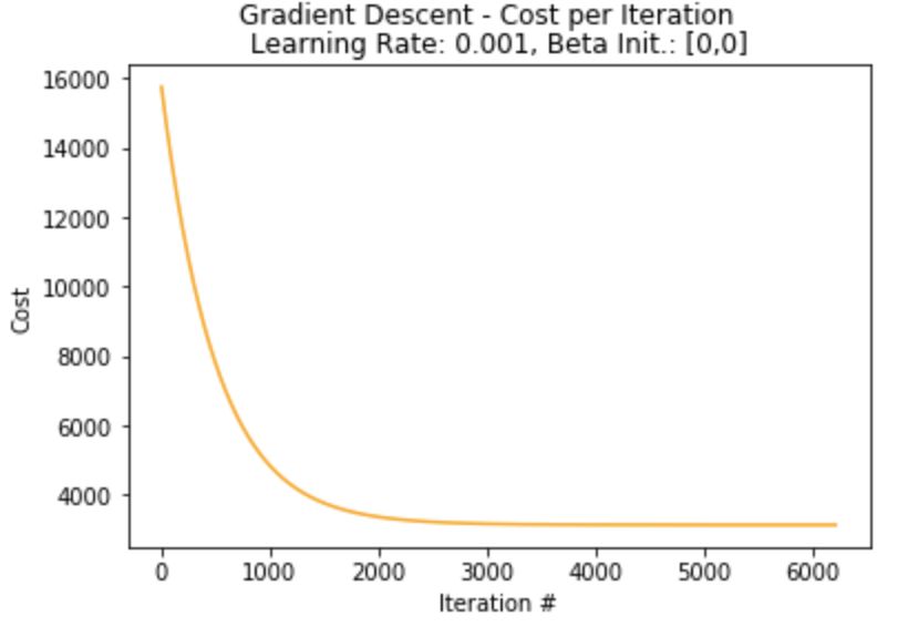
# defining plotting function
def plot_cost(cost,beta_init):
    plt.plot(range(len(cost)),cost,color="orange")
    plt.xlabel("Iteration #")
    plt.ylabel("Cost")
    plt.suptitle("Gradient Descent - Cost per Iteration")
    plt.title(str("Learning Rate: "+str(alpha)+", Beta Init.: "+str(beta_init)))
# plot single loss curves
plot_cost(cost_list_single,"[0,0]")
print("Lowest Loss: ",cost_list_single[-1])
Lowest Loss: 3136.304076502028

# plot multi loss curve
plot_cost(cost_list_single,"[0,0,0,0]")
print("Lowest Loss: ",cost_list_single[-1])
Lowest Loss: 3136.304076502028

Experiment with several initialisations: visualisation of the cost function and parameter values during the iterations
#-- Test 1  - simple reg
betas_list_single_init2,cost_list_single_init2 = grad_descent(
    X_train_single,y_train_single,beta_init=[100]*X_train_single.shape[1],alpha=alpha,iterations=20000,earlystop=True)

plot_cost(cost_list_single_init2,"[100,100]")
print("Lowest Loss: ",cost_list_single_init2[-1])
Loss stopped decreasing at iteration number:  5191
Lowest Loss:  3136.3040604978087

#-- Test 2 - multiple reg
betas_list_multi_init2,cost_list_multi_init2 = grad_descent(
    X_train_multi,y_train_multi,beta_init=[100]*X_train_multi.shape[1],alpha=alpha,iterations=20000,earlystop=True)

plot_cost(cost_list_multi_init2,"[100,100,100,100]")
print("Lowest Loss: ",cost_list_multi_init2[-1])
Loss stopped decreasing at iteration number:  11225
Lowest Loss:  2997.0782391353164

Notes: Expirimental setting, visualizations, explanations
Experiment with several learning rates: visualisation of the cost function and parameter values during the iterations
Learning Rate 0.001
#-- Test 1  - simple reg
betas_list_single_alpha2,cost_list_single_alpha2 = grad_descent(
    X_train_single,y_train_single,beta_init=[100]*X_train_single.shape[1],alpha=0.01,iterations=20000,earlystop=True)

plot_cost(cost_list_single_alpha2,"[100,100]")
print("Lowest Loss: ",cost_list_single_alpha2[-1])
Loss stopped decreasing at iteration number:  632
Lowest Loss:  3136.2589997697655

#-- Test 2 - multiple reg
betas_list_multi_alpha2,cost_list_multi_alpha2 = grad_descent(
    X_train_multi,y_train_multi,beta_init=[100]*X_train_multi.shape[1],alpha=0.01,iterations=20000,earlystop=True)

plot_cost(cost_list_multi_alpha2,"[100,100,100,100]")
print("Lowest Loss: ",cost_list_multi_alpha2[-1])
Loss stopped decreasing at iteration number:  1570
Lowest Loss:  2996.9034364503486

Learning Rate 0.0001
#-- Test 1  - simple reg
betas_list_single_alpha3,cost_list_single_alpha3 = grad_descent(
    X_train_single,y_train_single,beta_init=[0]*X_train_single.shape[1],alpha=0.0001,iterations=20000,earlystop=True)

plot_cost(cost_list_single_alpha3,"[0,0]")
print("Lowest Loss: ",cost_list_single_alpha3[-1])
Loss did not stop decreasing in 20000 iterations.
Lowest Loss:  3367.69870018736

betas_list_multi_alpha3,cost_list_multi_alpha3 = grad_descent(
    X_train_multi,y_train_multi,beta_init=[0]*X_train_multi.shape[1],alpha=0.0001,iterations=20000,earlystop=True)

plot_cost(cost_list_multi_alpha3,"[0,0,0,0]")
print("Lowest Loss: ",cost_list_multi_alpha3[-1])
Loss did not stop decreasing in 20000 iterations.
Lowest Loss:  3214.5086346029407

Notes
on the coice of learning rate
A low learning rate leads to very quick loss improvements, but is likely to substentially overshoot the target. Choosing a low learning rate significantly increases computing time, so that even after 20000 iterations the lowest loss was not yet reached. On the other hand, a small learning rate will get very closer to the best result, but it is questionable if the small improvement in accuracy is worth the significantly increased computing time.
on the choice of the stopping criterion:
In this case, as a stopping criterion a value of 0.0001 was chosen, representing the difference between the loss of the current iteration vs. the loss of the previous iteration. A problem is that if the learning rate is too high, we might overshoot the target, meaning the aforementioned difference is too high, leading to the last item in the list being acually the 2nd best approach. With a small learning rate on the other hand, it is unlikely to get into a negative value and even if we do so, the small learning rate only allows a small deviation.
on the data normalisation:
Normalozation is very important because the explanatory variables are in different scales. When normalized, they can be compared to each other. Additionally, chosing the right normalization method is vital because severe outliers might distort the range of values, leading to an unrepresentative date range.