Introduction
Using the semantic Earth Observation Data Cube Sen2Cube, the cloud cover of three different AOIs over the year 2019 is analysed.
The semantic query model builder functionality can create complex expressions by dragging and dropping blocks, which can select, adapt, perform dimension reduction and display the final result without coding at all.
Cloud cover percentage

<xml xmlns="http://www.w3.org/1999/xhtml"><block type="model_root" id="$UHM+5Y,)mHa=8;vJ*SA" deletable="false" x="256" y="19"><field name="name">Count Cloud Presence</field><statement name="semantic_concepts"><block type="entity_definition" id="rAh/mqJI($pwq0,nb;a["><mutation listlength="1"></mutation><field name="name">cloud</field><value name="item_0"><block type="property_definition" id="-J9)jf,(zhla4NjlTs*`"><field name="name">colour</field><value name="rules"><block type="compound" id=".o{e7gdr@n0bI=8lkjV{"><value name="with"><block type="atmosphere" id="=`3O]]!(y!!G[6CBr?WH"><field name="measurement">Color type</field></block></value><value name="do"><block type="evaluate" id="L[467mdPQhVz*[;C^$|W"><field name="operator">isin</field><value name="y"><block type="category" id="_=o+UgbL#F3Q2urCQXZK"><field name="category">CL</field></block></value></block></value></block></value></block></value></block></statement><statement name="application"><block type="result_definition" id="g-#IJqs0/71vhv7jW}.="><field name="name">cloud_count</field><field name="export">true</field><value name="instructions"><block type="compound" id="Oz]!5se#A,^OPA%1UmsE"><value name="with"><block type="entity" id="O)SqgoZ=}RpgorNAwr5P"><field name="name">cloud</field></block></value><value name="do"><block type="chain" id="J9o$cI/lLGgza|4OCq^c"><mutation listlength="1"></mutation><value name="item_0"><block type="reduce" id="NTw`@amg)N}#+_^osd6i"><field name="dimension">time</field><field name="operation">percentage</field></block></value></block></value></block></value></block></statement></block></xml> 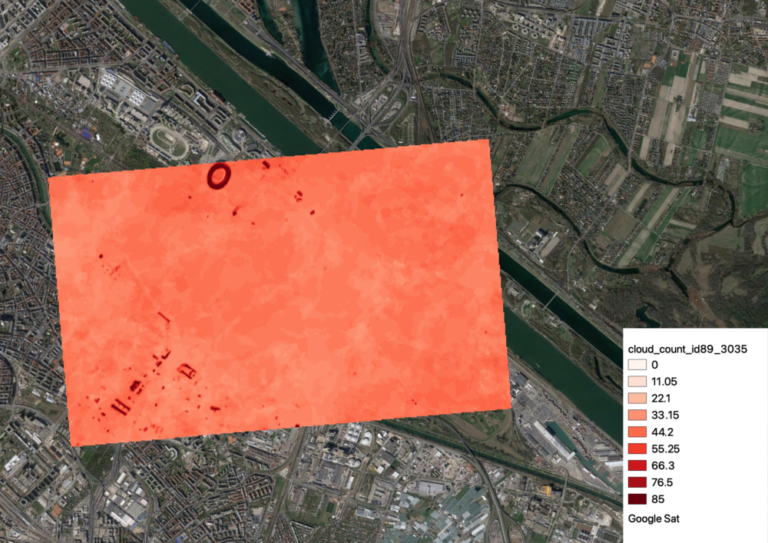
It makes sense that the cloud coverage over such a small area does not vary much from pixel to pixel. An interesting sidenote is, that the roof of the stadium as well as some other roofs in the South-West of the study area appear white and where thus almost always classified as cloud, with a much higher percentage than the surrounding area.
Cloud cover graphs
Since only an area of a certain size can be analyzed by percentage at once, but the value naturally does not vary much within the AOI, it is of interest to perform the same analysis at multiple locations.
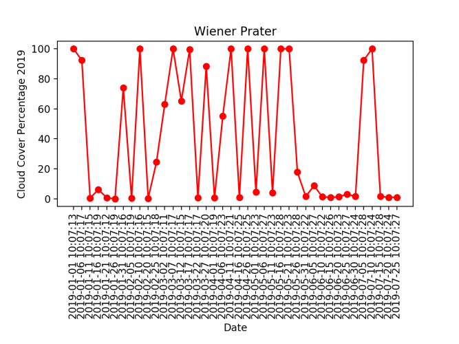
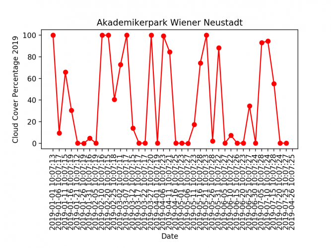
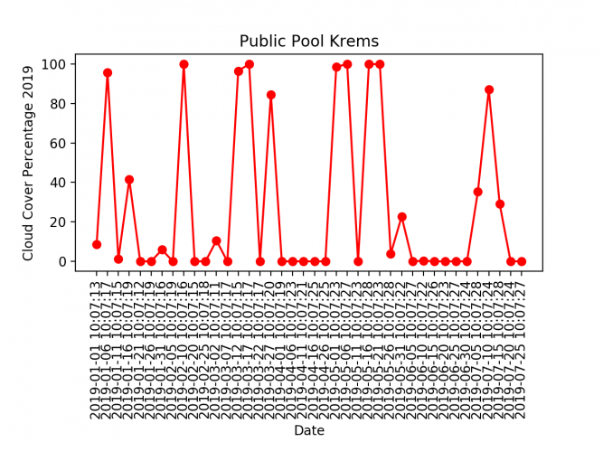
Reducing the data cube over space will eliminate the space dimension, leaving the time dimension and thus the output is a graph. This graph will show the development of cloud cover throughout the year. Other than the different reduction dimension, the other settings are kept the same as in the previous example. This will be performed at three locations:
- The Prater Recreational Park in Vienna
- The Akademikerpark in the Wiener Neustadt
- The Public Pool in Krems along the Danube
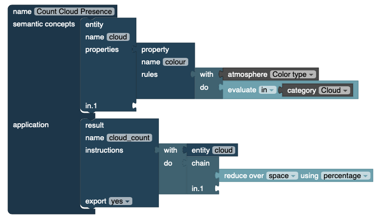
<xml xmlns="http://www.w3.org/1999/xhtml"><block type="model_root" id="$UHM+5Y,)mHa=8;vJ*SA" deletable="false" x="256" y="19"><field name="name">Count Cloud Presence</field><statement name="semantic_concepts"><block type="entity_definition" id="rAh/mqJI($pwq0,nb;a["><mutation listlength="1"></mutation><field name="name">cloud</field><value name="item_0"><block type="property_definition" id="-J9)jf,(zhla4NjlTs*`"><field name="name">colour</field><value name="rules"><block type="compound" id=".o{e7gdr@n0bI=8lkjV{"><value name="with"><block type="atmosphere" id="=`3O]]!(y!!G[6CBr?WH"><field name="measurement">Color type</field></block></value><value name="do"><block type="evaluate" id="L[467mdPQhVz*[;C^$|W"><field name="operator">isin</field><value name="y"><block type="category" id="_=o+UgbL#F3Q2urCQXZK"><field name="category">CL</field></block></value></block></value></block></value></block></value></block></statement><statement name="application"><block type="result_definition" id="g-#IJqs0/71vhv7jW}.="><field name="name">cloud_count</field><field name="export">true</field><value name="instructions"><block type="compound" id="Oz]!5se#A,^OPA%1UmsE"><value name="with"><block type="entity" id="O)SqgoZ=}RpgorNAwr5P"><field name="name">cloud</field></block></value><value name="do"><block type="chain" id="J9o$cI/lLGgza|4OCq^c"><mutation listlength="1"></mutation><value name="item_0"><block type="reduce" id="NTw`@amg)N}#+_^osd6i"><field name="dimension">space</field><field name="operation">percentage</field></block></value></block></value></block></value></block></statement></block></xml> The following graphs are the result of the Sen2Cube Query. The graphs have been produced in Python with the code below.
from matplotlib import pyplot as plt
import pandas as pd

csv_paths=['cloud_count_wien.csv','cloud_count_neustadt.csv','cloud_count_krems.csv']
title_lst=['Wiener Prater','Akademikerpark Wiener Neustadt','Public Pool Krems']

def charts(path,title):
    df = pd.read_csv(path)
    plt.figure()
    plt.plot( 'time', 'cloud_count', data=df, marker='o', color='red')
    plt.xticks(df1['time'], rotation='vertical')
    plt.subplots_adjust(bottom=0.4)
    plt.xlabel('Date')
    plt.ylabel('Cloud Cover Percentage 2019')
    plt.title(title)
    plt.savefig(path[:-4]+'.png',dpi=200)


for path,title in zip(csv_paths,title_lst):
charts(path,title) 

