


The M.Sc. thesis was resarched, written and defended at the University of South Brittany in Vannes, France between Februrary and June 2022.
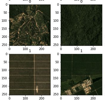
Several predefined deep learning computer vision models, such as LeNet, ResNet18, VGG16 and AlexNet are used to identify palm oil plantations in satellite images. The models are both trained from scratch and used as a feature extractor via transfer learning on the pretrained models.
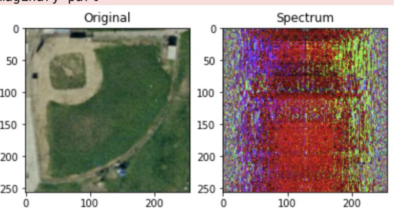
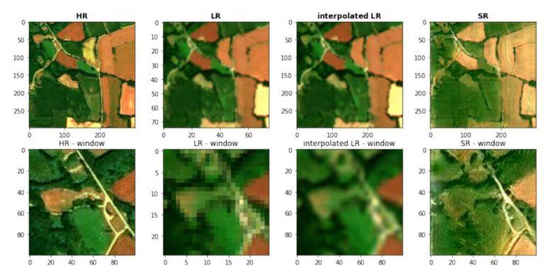
Performing some Fourier Transformations and filtering operations on images.