River Catchment – Tasks

In this exercise, a river catchment area is analyzed regarding its slope and curvature. The following tasks are performed:

  • Slope Visualization, Statistics and Histogram for the whole catchment area
  • Analyze the slope and it’s statistics for different elevation zones within the catchment area
  • Comparing slope statistics for 10m and 100m spatial resolution
  • Calculating curvature without the “curvature” function in ArcGIS Pro


Study Area

As a study area, the Neubach catchment area was chosen. This little river originates in the mountains of the Dachstein massif and its slopes, before feeding into the Lammer which eventually feeds into the Salzach near Golling an der Salzach.

Image 1: Location of the study area in relation to Salzburg. Study area is already visualized as DEM.
Image 2: 3D Hillshide visualization of the catchment area. The red zones deliniate the multiple catchment areas that eventually drain into the Neubach.

For the analysis, seven separated catchment areas were unified. Those areas all have the same exit point, where the Neubach drains into the Lammer. The Catchment Code (HZB_CODE) unifies those areas under the code 2-8272231-14.

The study area ranges from 850m in elevation at the drainage point until just over 2000m on the flank of the Dachstein massif.

Slope – complete Catchment Area

From the DEM, the slope per pixel is calculated in degrees. Also, a histogram is created in Python (the code can be found at the end of the post) that shows the slope of the whole study area in 5° steps as well as the mean value.
Click right on the slideshow to see the Histogram

Elevation Zone Creation

Next up, the catchment area is devided into the following four elevation zones:

  • <1000m
  • 1000 – 1250m
  • 1250 – 1500m
  • 1500 – 1750m
  • > 1750m

Slope per Elevation Zone

Now, the slope average and histogram are calculated for each elevation zone.

The average slope for the different elevation zones are as follows:

  • <1000m: 19.3°
  • 1000 – 1250m: 25.6°
  • 1250 – 1500m: 32.3°
  • 1500 – 1750m: 25.5
  • > 1750m: 34.9

Interestingly, the slope does not always increase the higher up the mountain you go. Zone 4 (1500 – 1750m) has a lower average slope with 25.5°, most likely doe to the flatter area in the northern zone as well as the mountain ridge in the southern area of this zone.

This observation is supported if a profile graph is drawn across all elevation zones.

Resampling to 100x100m Slope Pixels

Now, the slope .tiff is resampled to a pixel size of 100 by 100 meters to see if the slope averages change depending on the spatial resolution of the underlaying data.

Image 13: 100x100m Resampled Slope Visualization.
Table 1: Comparison of average slope per Elevation Zone and spatial resolution.

Comparing the average slopes of the different elevation zones and spatial resolutions shows that the average slope does not drastically change. As a resampling algorithm to downsample the images, the bilinear method was chosen. The low difference indicates that this method yielded good results. Surely, if another resampling method such as Nearest Neighbor would have been chosen, the result would have been much less acurate.

Curvature calculation without ArcGIS curvature function

Calculating the curvature of an area is very simple with the curvature function in ArcGIS Pro, but there is another easy workaround. Since we already have the slope layer, which indicates the slope of each pixel, we can run the slope function again on the same dataset.

After the first execution, the values show the slope of the pixel. Since the curvature is the second derivative of the slope (slope-of-the-sope), the result is similar to the curvature function.

The curvature function results in pixel values from ca. -4 to 4, while the slope of the slope is still in degrees. The degrees can be scaled to the same values, which results in the same output. Unfortunately, the visualization is different for the following two curvature representations, but the areas of conformity are still visible. Clearly, the two images show the same real-life phenomenon.

Finally, as anounced, here is the code used to create all histograms in this post.

#!/usr/bin/env python3
# -*- coding: utf-8 -*-

import numpy as np
import matplotlib.pyplot as plt
from PIL import Image
# Also open large images
Image.MAX_IMAGE_PIXELS = None

paths_slopes_resample=[
"slope_1000_resampled.tif",
"slope_1250_resampled.tif",
"slope_1500_resampled.tif",
"slope_1750_resampled.tif",
"slope_2050_resampled.tif",
]

paths_slopes=[
"slope_1000.tif",
"slope_1250.tif",
"slope_1500.tif",
"slope_1750.tif",
"slope_2050.tif",
]

path_slope_10 = ["slope_complete.tif"]
path_slope_100 = ["slope_complete_100.tif"]


# create clean title names from path
def extract_title(path):
    name = path[:-4]
    if "resample" in name:
        name = name.replace("_resampled",", 100x100m")
    else:
        name = name+", 10x10m"
    name = name.replace("_"," ")
    name = name.replace("s","S")
    name = name.replace("r","R")
    name = name.replace("Slope","Slope in Degrees,")
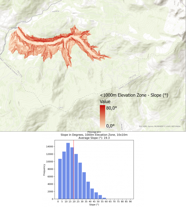
    name2 = name[:22]+"m Elevation Zone"+name[22:]
    return(name2)

# Opening Image path, converting to numpy array, deleting nan values
def to_np(path):
    im = Image.open(path)
    im_array = np.array(im)
    # round values to 2 decimal places
    im_array = np.round(im_array, 2)
    #Remove 0 (null) values
    im_array[im_array == 0] = np.nan
    # Remove nan values
    im_array = im_array[~np.isnan(im_array)]
    im_array = im_array[np.logical_not(np.isnan(im_array))]
    
    #print((im_array))
    return im_array


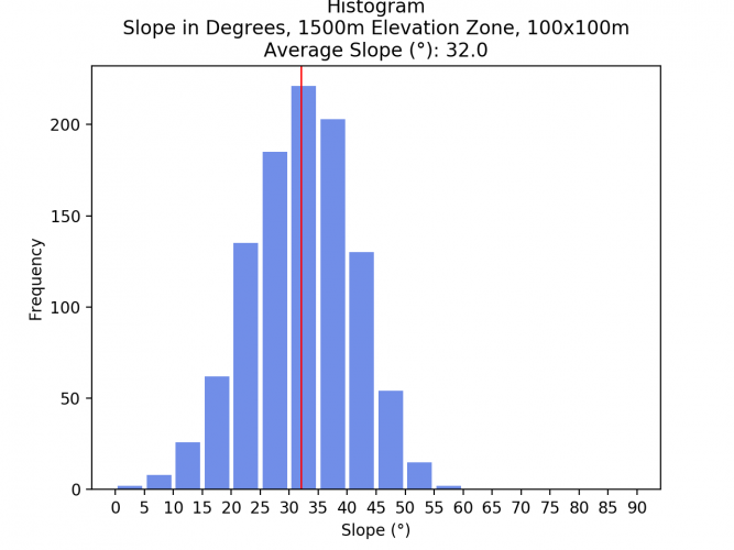
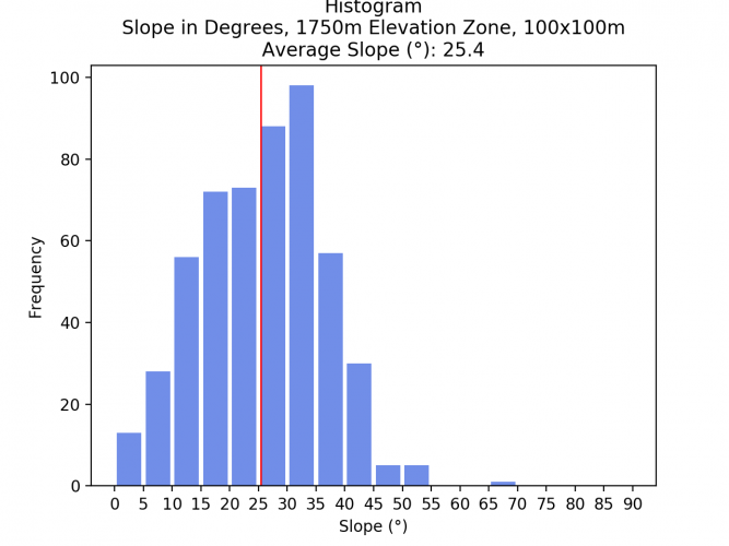
def graph(im_array,path,name):
    # setting bns in 5 degree steps
    bins=[0,5,10,15,20,25,30,35,40,45,50,55,60,65,70,75,80,85,90]
    # draw histogram
    n, bins, patches = plt.hist(im_array[~np.isnan(im_array)], bins=bins,color="royalblue", alpha=0.75, rwidth=0.85)
    #set y grid
    #plt.grid(axis='y', alpha=0.75)
    # calculate mean
    im_mean = im_array[~np.isnan(im_array)].mean()
    # add mean line
    plt.axvline(im_mean, color='red', linestyle='solid', linewidth=1)
    # Set ticks, labels and title
    plt.xticks(bins)
    plt.xlabel("Slope (°)")
    plt.ylabel('Frequency')
    plt.title('Histogram\n'+name+"\nAverage Slope (°): "+str(round(im_mean,1)))
    #set output name to sth computer readable and save
    output_name = "histograms/"+path[:-4]+"_histogram.png"
    plt.savefig(output_name,dpi=200)
    print("saved: ",output_name)
    # clear figure after saving
    plt.clf()
    plt.close("all")


for path in paths_slopes:
    graph(to_np(path),path,extract_title(path))

for path in paths_slopes_resample:
    graph(to_np(path),path,extract_title(path))

#Warning: Overflow in mean calculation possible
for path in path_slope_10:
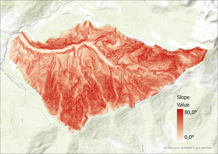
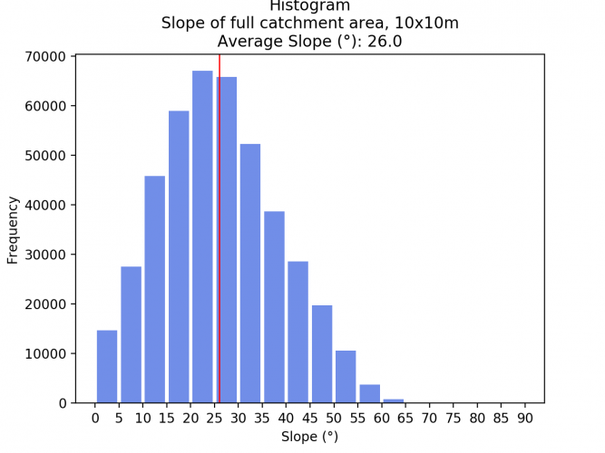
    graph(to_np(path),path,"Slope of full catchment area, 10x10m")

for path in path_slope_full:
    graph(to_np(path),path,"Slope of full catchment area, 100x100m") 

Leave a Reply

Your email address will not be published. Required fields are marked *

Further Reading
Recent Updates